Origins of Neural Networks
Artificial Neural Networks
Artificial Neural Networks
An artificial neural network (ANN) is a computing system that is similar to a biological neural network. These systems learn to do tasks by considering examples, generally without task-specific programming.
June 23, 2017—Aishwarya Praveen
Warren McCulloch and Walter Pitts created a computational model for neural networks based on mathematics and algorithms called threshold logic. This led to research for neural network splitting into two approaches; one was focused on the biological processes in the brain, while the other focused on the application of neural networks to artificial intelligence (AI).
In 1958, Rosenblatt created the perceptron, an algorithm for pattern recognition. With mathematical notation, Rosenblatt described circuitry not in the basic perceptron, such as the exclusive-OR circuit.
Neural network research stagnated after machine learning research by Minsky and Papert, who discovered two key issues with the computational machines that processed neural networks. The first was that the basic perceptrons were incapable of processing the exclusive-OR circuit. The second was that computers didn’t have enough processing power to effectively handle the work required by large neural networks. Neural network research slowed until computers achieved far greater processing power.
Neural Net Layers
Neural Net Layers
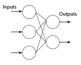
The neurons are organized in layers where the signals travel from a set of inputs to the last set of outputs after traversing successively all the layers.
Let’s have a look at the topology of the network:
In[]:=
Import["http://neuroph.sourceforge.net/tutorials/images/perceptron.jpg","Image"]
Out[]=
In the Wolfram Language, we can use the NetGraph symbol. It can be used to specify a neural net defined by a graph in which the output of layer is given as input to layer .
m
i
n
i
Create a net with one layer:
In[]:=
neuralnet=NetGraph[{ElementwiseLayer[Ramp]},{}]
Out[]=
NetGraph
Create a net with two layers whose output vectors are 3 and 5:
In[]:=
net=NetGraph[{LinearLayer[3],LinearLayer[5]},{12},"Input"2]
Out[]=
NetGraph
Initialize all arrays in the above net and give numeric inputs to the net:
In[]:=
net=NetInitialize[net];
In[]:=
net[{1.0,2.0}]
Out[]=
{-0.541849,-0.167301,-0.0138126,-0.338522,-0.549727}
Create a linear layer whose output is a length-5 vector:
In[]:=
LinearLayer[5]
Out[]=
LinearLayer

The above linear layer cannot be initialized until all its input and output dimensions are known. The LinearLayer is a trainable, fully connected net layer that computes only the output vector of size n.
Create a randomly initialized LinearLayer:
Create a randomly initialized LinearLayer:
In[]:=
linear=NetInitialize@LinearLayer[5,"Input"3]
Out[]=
LinearLayer
In[]:=
linear[{1,2,1}]//MatrixForm
Out[]=
-0.741161 |
-0.867255 |
-0.843027 |
1.48873 |
0.266249 |
The linear function was used to call three inputs that gave a matrix vector of five elements, i.e because we initialized a linear layer of five outputs.
In[]:=
Import["https://www.researchgate.net/profile/Haohan_Wang/publication/282997080/figure/fig4/AS:305939199610886@1449952997594/Figure-4-A-typical-two-layer-neural-network-Input-layer-does-not-count-as-the-number-of.png","Image"]
Out[]=
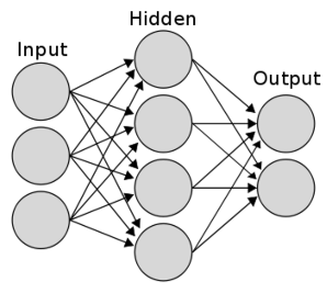
The above is a representation of a two-layer neural network.
Let’s make our own neural network and use that to classify the MNIST handwritten digits. We will first load the data, and we will take 5,000 examples as training data and 1,000 examples as test data:
In[]:=
resource=ResourceObject["MNIST"];trainingDataImg=RandomSample[ResourceData[resource,"TrainingData"],5000];testDataImg=RandomSample[ResourceData[resource,"TestData"],1000];
In order to train the example, we take the pixel values of the image and flatten them into a list; as for the digits, we change them into 10x1 vectors, with the corresponding index setting to be 1.
In[]:=
rule=Rule[x_,y_]:>Flatten[ImageData[x]]->(If[#==y+1,1,0]&/@Range[10]);trainingData=trainingDataImg/.rule;testData=testDataImg/.rule;
Now we can construct the neural network. We will use three layers of (28*28), 30 and 10 neurons. Each neuron will be activated by the sigmoid function:
In[]:=
lenet=NetChain[{(*secondlayer*)DotPlusLayer[30],ElementwiseLayer[LogisticSigmoid],(*thirdlayer*)DotPlusLayer[10],ElementwiseLayer[LogisticSigmoid]},"Input"784]
Out[]=
NetChain
Let’s train this!
In[]:=
trained=NetTrain[lenet,trainingData,MaxTrainingRounds150]
Out[]=
NetChain
Let’s test it out!
In[]:=
Counts[testData/.Rule[x_,y_]First@Flatten[Position[#,Max[#]]&@trained[x]]-1First@Flatten@Position[y,1]-1]
Out[]=
False110,True890
We get an accuracy of 89% with a three-layer neural network.
Convolutional Neural Network
Convolutional Neural Network
Convolutional Layer
Convolutional Layer
Pooling Layer
Pooling Layer
FURTHER EXPLORATIONS
Recurrent Neural Networks
Differentiable Neural Computers
AUTHORSHIP INFORMATION
Aishwarya Praveen
6/23/17