Universal Function Approximation Using Neural Networks
Universal Function Approximation Using Neural Networks
Numerical approximation of functions by hand can be time consuming, and can require a lot of manual analysis. However, given a large sample of input and output values, neural networks are capable of approximating nearly any continuous, real-valued function. This is a simple example of using Mathematica to train a multilayer perceptron (MLP), utilizing a logistic sigmoid activation function. MLPs use an algorithm called backpropagation, which enables it to model the coefficients that best approximate a function while minimizing error.
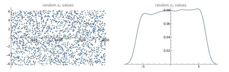
Sample GenerationFirst, we need to generate the input values that we will use to train our model. To do so, we will define some random values ∈ X
x
On[Assert](*setthesamplesizehere*)n=2000;(*defineourdatageneratorfunction--nnumberofpseudorandomreals,chosenfromauniformprobabilitydistributionwithintherangespecified*)generateRandomData[n_,range_]:=RandomReal[range,n](*defineourplottingfunction*)plotTestData[testdata_]:=GraphicsGrid[{{ListPlot[testdata,PlotLabel"random values",ImageSizeMedium],SmoothHistogram[testdata,PlotLabel"random values"]}}](*nowwecangenerateasample,andplottheresults*)testdata=generateRandomData[n,{-2*π,2*π}];plotTestData[testdata](*belowwecanverifythatthedataappeartobewelldistributed*)
x
n
x
n
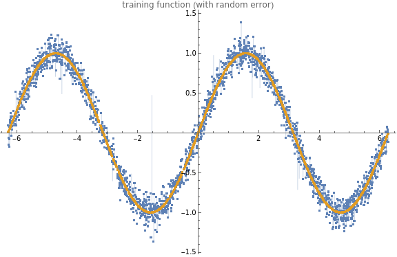
Evaluate Sample DataNow that we have a lot of random values, we can evaluate them through an arbitrary function to get observed values, which we will use to “teach” our network.But first, let’s make it more challenging by adding a little Gaussian noise to our output, to muddy the waters a bit (because nothing in life is ever perfect).
x
(*definenoisegenerationfunction--thiswilladdsomerandomnoisetoagenericdataset*)noisify[data_]:=data+(.1*Normal[RandomFunction[WhiteNoiseProcess[],{0,Dimensions[data][[1]]-1}]][[1]][[All,2]]);(*definedelegatefortrainingfunction,tobeusedlater*)trainingfunction[x_,func_]:=noisify[func[x]];
Now, the function: we can choose anything here, but let’s use something tricky, such as a trigonometric function:.
Let’s go ahead and see what our noisy function looks like to make sure we haven’t added too much error.
Now, the function: we can choose anything here, but let’s use something tricky, such as a trigonometric function:
sin(x)
Let’s go ahead and see what our noisy
sin(x)
(*buildahelpermoduletovisualizetestdata--thiswillplotthedata(anditserror)alongwithareferencelineoftheoriginalfunction*)visualizeTestData[data_,dataClean_]:=Module[{},ListPlot[{data,dataClean},PlotLabel"training function (with random error)",ImageSizeLarge,Filling{1{2}},PlotLegendsPlaced[{"training function (with random noise)","perfect function (for reference)"},Right]]](* *evaluateourrandomsamplethroughthe"noisified"function*alsoevaluateoursamplethrougha"non-noisy"versionofthefunction(forcomparison)*)buildTestData[testdata_,func_]:=Module[{y,yclean},(*evaluatedirty*)y=Evaluate[trainingfunction[testdata,function]];(*evaluatenon-dirty*)yclean=Evaluate[function[testdata]];(*nowweneedtopairthexandyvaluesforeachresult*)dataPairs=Transpose@{testdata,y};dataPairsClean=Transpose@{testdata,yclean};](*FINALLYwedefineouractualfunction*)function=Sin;buildTestData[testdata,function];visualizeTestData[dataPairs,dataPairsClean](*Belowwecancheckoutourxandysamples,inthecharacteristic"sin"wavewithsomeslighterroraddedforrealism*)
Build Training SetNow that we are confident with our sample data, and our function results, we can organize the paired samples into distinct classes for training and validation sets. We will use two of these sets to train the MLP (a training set to learn the estimation function, and a cross-validation set to help optimize the weights), and a third setwill be used for testing and evaluation purposes.
(*first,let'sdefineacoupleofgetterstoaccessourdatapairs*)getInput[list_]:=First/@list;(*getinputvalues(x)*)getOutput[list_]:=Last/@list;(*getoutputvalues(y)*)(*"split"moduletorandomlysampleaproporationofourdata*)split[]:=Module[{input,output,trainingthreshold,random},input=dataPairs[[All,1]];output=dataPairs[[All,2]];SeedRandom[1234];random=RandomSample[Transpose[{input,output}]];trainingthreshold=Floor[0.7Length[input]];validationthreshold=Floor[.9Length[input]];training=random[[;;trainingthreshold]];validation=random[[trainingthreshold+1;;validationthreshold]];(*thisthirdsetwillremainunseenuntilevaluationstage*)test=random[[validationthreshold+1;;]];]; split[];
Let’s do a quick check of our distributions and make sure that everything still looks nice and random.
Let’s do a quick check of our distributions and make sure that everything still looks nice and random.
Neural Network Training
Now we can train the MLP itself. Mathematica has made this really simple as of Mathematica 11, including cross-validation. We are going to use a standard
logistic function for the network’s activation function, of which much as been written. This makes a more effective prediction than standard linear models, in that it is both non-linear and only delivers
values between 0 and 1, which is convenient when dealing with binomial trials and binary classification tasks (such as true/false).
Generalizing
Generalizing
Now we can view our training sample, and visualize the random error we have introduced, displayed on top of a perfect Cos wave.
And another split of the data, to make sure our data is still nice and evenly distributed.
Now our model can learn the new function, and we can view it’s performance against our held-out “unseen” values. Still looks pretty good!
Try it yourself:
One more experiment: let’s demonstrate the loss of precision and accuracy as we extend our extrapolation beyond the range of the initial training set. It becomes clear that as we depart out 2π range, our model quickly loses discriminative power. Neat, right? Be careful to avoid extrapolation!