Wolfram Language
Wolfram Language
For Mathematics Computation
Overview
Overview
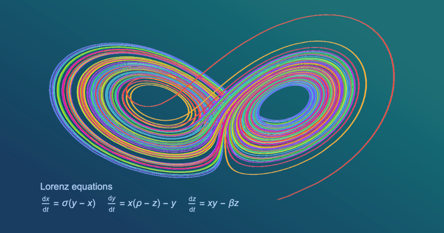
Wolfram Language has extensive capabilities for doing mathematics both symbolically and numerically. This presentation will cover:
Algebra and Calculus
Solving Equations
Linear Algebra
Function Visualization
Equation Solving
Solving Differential Equations
PDE Examples
Algebra and Calculus
Algebra and Calculus
The Wolfram Language has all that you need for working with and manipulating mathematical expressions.
Algebraic Manipulations
Algebraic Manipulations
The Wolfram Language uses a wide range of transformations to simplify complicated mathematical expressions.
Simplifying algebraic and trigonometric expressions
Simplifying algebraic and trigonometric expressions
In[]:=
FullSimplify-+
1
3(1+x)
-1+2x
6(1-x+)
2
x
2
31+
1
3
2
(-1+2x)
In[]:=
FullSimplify[-1+50-400+1120-1280+512]
2
Cos[x]
4
Cos[x]
6
Cos[x]
8
Cos[x]
10
Cos[x]
Simplifications involving special functions
Simplifications involving special functions
In[]:=
FullSimplify[Gamma[x]*Gamma[1-x]]
Collecting terms involving x
Collecting terms involving x
In[]:=
Collect[(1+a+x)^4,x]
Eliminate a variable from a system of equations
Eliminate a variable from a system of equations
In[]:=
Eliminate[2x+3y+4z1&&9x+8y+7z2,z]
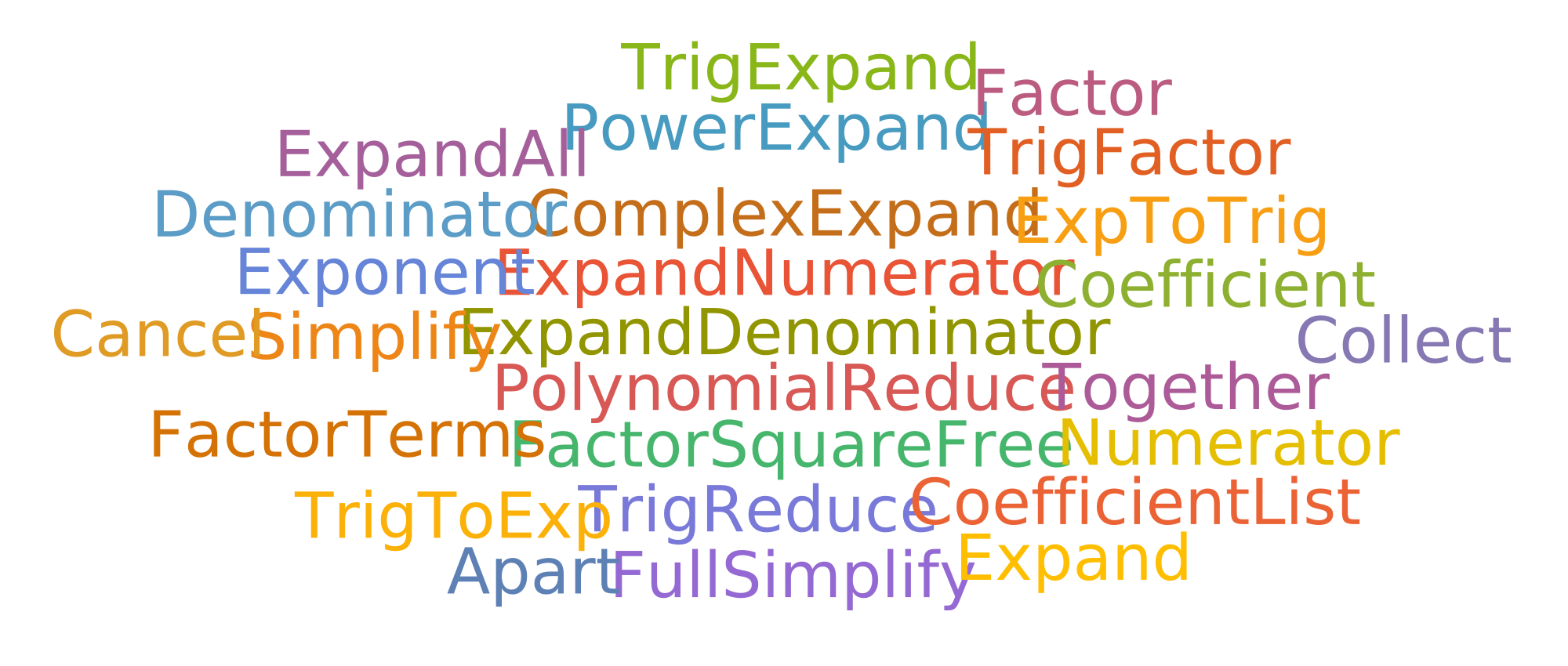
It would take an entire section or more to demonstrate the full power of the Wolfram Language for symbolic manipulation of mathematical expressions. The following contains many functions for doing such manipulations. Clicking a particular word will bring you to the documentation page of that function:
Limits
Limits
Sums
Sums
Differentiation
Differentiation
Symbolic Integration
Symbolic Integration
Numeric Integration
Numeric Integration
Solving Equations
Solving Equations
The Wolfram Language can solve equations and systems of equations in symbolic form.
Below we are finding where the curve=xy+1 intersects a circle of radius 2 centered at {1,1}, but only within the region defined by the circle of radius 2 centred at {0,0}. While the solution is given in term of Root functions, a numerical result can be obtained with the N function.
Below we are finding where the curve
2
x
ℛ
1
ℛ
2
ℛ
3
ℛ
1
ℛ
2
2
x
ℛ
3
Visualize the result.
In[]:=
Show[{ContourPlot[xy+1,{x,-2,3},{y,-2,3},ContourStyle{Black},FrameLabel{x,y},PlotTheme"Presentation"],Graphics[{{Hue[.125,1,1,.3],},{ColorData[106,4],Thick,},{ColorData[106,3],PointSize[0.03],Point[{x,y}/.sol]}}]}]
2
x
ℛ
1
ℛ
2
Conditional expressions are used if the solution depends on the values of the parameters
In[]:=
Solve[x^2+ax+b0,x,Reals]
General polynomial equations can be solved in terms of Root functions, while a numerical result can be obtained with the N function
In[]:=
Solve[x^5-2x+170,x]N[%]
Systems of equations can be solved:
In[]:=
Solve[{x+2y+3z4,3x+4y+5z6,7x+7y+8z9},{x,y,z}]
Inequalities can be used to constrain the region of valid solutions
Solve omits solutions involving equations on parameters. If you want these extra equations, use Reduce.
The Wolfram Language is able to solve recurrence equations in a general form:
Initial conditions on the recurrence equation can also be specified:
Linear Algebra
Linear Algebra
The Wolfram Language includes an wide range of operations for doing linear algebra.
Along with the basic operations, the Wolfram Language also included many matrix decompositions.
Function Visualization
Function Visualization
The Wolfram Language incorporates advanced algorithms to automate the immediate creation of highly aesthetic and technically correct 2D and 3D visualizations.
Basic Plots
Basic Plots
Plots of a single variable:
Plots of a single variable:
Plots with two variables:
Plots with two variables:
Complex Plots
Complex Plots
A complete listing of the functions available can be found in the Function Visualization guide page.
Equation Solving
Equation Solving
The Wolfram Language includes a number of functions for solving equations and inequalities.
Solve can also be provided with a series of inequalities to constrain the solution.
Application: Quantum Tunneling
Application: Quantum Tunneling
Answer: The form of the wave functions in the three regions is given by:
The task is to determine the coefficients. To do this, match the wave functions and their derivatives at each boundary. This sets up a system of equations that needs to be solved to determine the remaining coefficients.
Define some parameters.
Calculate the transmission coefficient by eliminating the other coefficients from the equations.
Solve for f, and calculate the transmission coefficient, which gives the probability that the wave will make it through the barrier.
The reflection coefficient is determined from the coefficient b. We could calculate it from T+R=1, but just because it is so easy, let’s eliminate the coefficients {c, d, f} from the equations.
Solving Differential Equations
Solving Differential Equations
Wolfram Language can solve a wide range of differential equations both symbolically and numerically.
Symbolic Solutions
Symbolic Solutions
Linear ODEs:
Linear ODEs:
Coefficients can be symbolic quantities:
Nonlinear ODEs:
Nonlinear ODEs:
DSolve is able to find symbolic solutions to a wide range of nonlinear ODEs.
When necessary, solutions will be given in terms of special functions.
System of Equations:
System of Equations:
When solving a system of equations, simply give DSolve the list of equations and dependent variables.
Differential Algebraic Equations (DAEs):
Differential Algebraic Equations (DAEs):
DAEs are differential equations that contain algebraic constraints as part of the system of equations:
Partial Differential Equations:
Partial Differential Equations:
Simply give the list of equations and conditions to DSolve to obtain the solution to the PDE.
Nonlinear PDEs:
Nonlinear PDEs:
DSolve can solve some nonlinear PDEs symbolically.
FEM Example: Wave in a pool
FEM Example: Wave in a pool
NDSolve uses the Finite Element Method (FEM) when solving partial differential equations over arbitrarily shaped regions. A complete discussion of using FEM with NDSolve can be found in the Finite Element Method User Guide.
Problem: Solve the wave equation in a pool with three rectangular regions taken out.
Answer: First set up the region.
Define the wave equation.
Specify the initial conditions of the wave packet.
Use DirichletCondition to specify that the function goes to zero on all boundaries.
Obtain a numeric solution to the problem.
Visualize the evolution of the solution over time.
Obtaining Material Constants
Obtaining Material Constants
Consider the flow of glycerol through a narrowing tube.
First, set up and visualize the geometry:
Specify the fluid flowing through the tube.
Here the chemical entity for glycerol is used to extract material properties.
Set up the fluid flow PDE component:
Set up boundary conditions:
Solve the PDE:
Visualize the fluid velocity:
Outlook
Outlook
Wolfram Language has numerous additional mathematical functions that could not be covered in this presentation.
The word cloud below contains a small collection of the mathematical functions, with 1000+ additional math functions available. Click on the respective name to get to the function’s documentation page.
Wolfram Language also contains advanced functionality in several other areas of mathematics, among these:
Wolfram Language also contains advanced functionality in several other areas of mathematics, among these:
Wolfram Research offers further mathematical resources online. Click any image to access the corresponding website.
Additional Resources
Additional Resources
Some useful links:
Wolfram U (videos and other resources in Wolfram Language)
Wolfram Demonstrations Project (example code for your domains)
Wolfram Community (discussion with peers)
WolframTechnical Support (the place to get your questions answered)