In[]:=
(*deployswithcanonicalname*)deploy:=Module[{notebookFn,parentDir,cloudFn,result},Print[DateString[]];notebookFn=FileNameSplit[NotebookFileName[]][[-1]];parentDir=FileNameSplit[NotebookFileName[]][[-2]];cloudFn=parentDir~StringJoin~"/"~StringJoin~notebookFn;result=CloudDeploy[SelectedNotebook[],CloudObject[cloudFn],Permissions"Public",SourceLinkNone];Print["Uploading to ",cloudFn];result];deploy
Thu 2 Mar 2023 16:48:43
Loss trajectory of quadratic with eigenvalues following semicircle law
Loss trajectory of quadratic with eigenvalues following semicircle law
accompanying mathematica.SO:
https://mathematica.stackexchange.com/questions/281808/improving-quality-of-plot-with-bad-numeric-performance
https://mathematica.stackexchange.com/questions/281808/improving-quality-of-plot-with-bad-numeric-performance
For semi-circle graph CDF, see
https://www.wolframcloud.com/obj/yaroslavvb/newton/forum-bernoulli-graphs.nb
https://www.wolframcloud.com/obj/yaroslavvb/newton/forum-bernoulli-graphs.nb
In[]:=
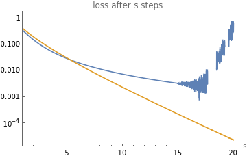
interval[var_,min_,max_]:=HeavisideTheta[var-min]-HeavisideTheta[var-max];{xmin,xmax}={0,1};xvals=Range[xmin,xmax,(xmax-xmin)/10];icdf[y_]=InverseCDF[WignerSemicircleDistribution[1],y]//Refine[#,0<y<1]&;g[x_]=icdf[(1-x/2)];(*reversesort,map0.5->1rangeto0..1*)ymin=Limit[g[x],x->xmax];ymax=Limit[g[x],x->xmin,Direction"FromAbove"];gi[y_]=First@SolveValues[{g[x]==y,xmin<x<xmax},x,Assumptions{ymin<y<ymax}];arg=-D[gi[y],y]*y;fwd=LaplaceTransform[arg*interval[y,ymin,ymax],y,s]/.s->2s;loss0=Asymptotic[fwd,s->0];loss=fwd/loss0//Simplify;Print["normalized loss after s steps=",loss];loss2=(Gamma[0,(2s)/5]-Gamma[0,2s])/Log[5];LogPlot[{loss,loss2},{s,1,20},PlotLabel->"loss after s steps",AxesLabel->{"s"},PlotLegends->{"random quadratic","harmonic decay"}]
normalized loss after s steps=(4-3πsBesselI[0,2s]+3πBesselI[1,2s]-3πsBesselI[2,2s]+3πsStruveL[0,2s]-3πStruveL[1,2s]+3πsStruveL[2,2s])
1
8
2
s
2
s
Out[]=