In[]:=
Tue 16 May 2023 10:53:51
Approximating solution of ∂∂tfhf+hdihf
Approximating solution of fhf+hdihf
∂
∂t
Solution has a simple form in Laplace Domain in terms of (No closed form in time domain , hence try asymptotic approximationsRelated questions:- “Simplifying arctan expression using Puiseux series” math.SE post Lutz recommended replacement, Goncalo provided expression from (x)≃x equivalence - “Solving ....” math.SE post DinosaurEgg gives ( solution by some algebra on the self-consistent equation- “When to use Series vs Asymptotic” mathematica.SE postParent notebook:forum-mean-field-equations.nb
-1
tan
s
)x=2
2
s
-1
tan
-1
tan
s
)Asymptotic expansions of ArcTan expression
Asymptotic expansions of ArcTan expression
In[]:=
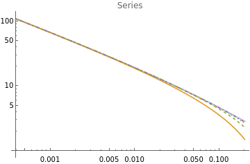
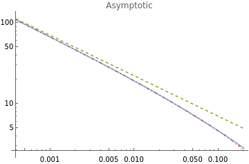
ClearAll["Global`*"];expr=+;SF=StringForm;series[order_]:=Normal@Series[expr,{s,0,order}];asymp[order_]:=Asymptotic[expr,{s,0,order}];{approxSeries,approxAsymp}=Table[{i,#[i]},{i,0,3}]&/@{series,asymp};visualize[approx_,label_]:=(Print[TableForm[approx,TableHeadings->{{},{"order","expr"}}]];LogLogPlot@@{{expr}~Join~(Last/@approx),{s,0.,.2},PlotLegends->{"true"}~Join~(SF["order ``",First@#]&/@approx),PlotStyle->{{Thick,Opacity[.5]},Automatic,Dashed,Dotted,DotDashed},PlotLabel->label})Quiet[visualize[approxSeries,"Series"]]Quiet[visualize[approxAsymp,"Asymptotic"]]
1
s
2
2
s
π-2ArcTan
s
2

order | expr | |
0 | 1 4 2 π π 2 s | |
1 | 1 4 2 π π 2 s π(8+ 2 π s 8 2 1 96 2 π 4 π | |
2 | 1 4 2 π π 2 s π(8+ 2 π s 8 2 1 96 2 π 4 π π(112+48 2 π 4 π 3/2 s 192 2 (-512-1200 2 π 4 π 6 π 2 s 3840 | |
3 | 1 4 2 π π 2 s π(8+ 2 π s 8 2 π- 2 3π 3π 4 2 3 π 16 2 2 π 7 12 2 π 4 4 π 64 3/2 s 2 π- 2 2 15π 5π 8 2 5 3 π 32 2 5 π 128 2 2 s 2 π 3 10 13 2 π 48 3 4 π 64 6 π 512 5/2 s 2 π- 29 315 2 π33π 80 2 5 3 π 24 2 7 5 π 256 2 7 π 1024 2 3 s 2 |
Out[]=
order | expr | |
0 | Asymptotic 1 s 2 2 s π-2ArcTan s 2 | |
1 | π 2 s | |
2 | 1 4 2 π π 2 s π(8+ 2 π s 8 2 1 96 2 π 4 π π(112+48 2 π 4 π 3/2 s 192 2 (-512-1200 2 π 4 π 6 π 2 s 3840 | |
3 | 1 4 2 π π 2 s π(8+ 2 π s 8 2 π- 2 3π 3π 4 2 3 π 16 2 2 π 7 12 2 π 4 4 π 64 3/2 s 2 π- 2 2 15π 5π 8 2 5 3 π 32 2 5 π 128 2 2 s 2 π 3 10 13 2 π 48 3 4 π 64 6 π 512 5/2 s 2 π- 29 315 2 π33π 80 2 5 3 π 24 2 7 5 π 256 2 7 π 1024 2 3 s 2 |
Out[]=
Do x=22s replacement
Do replacement
x=2
2
s
In[]:=
ClearAll["Global`*"];$Assumptions={x>0};expr=Simplify+/.s->2;SF=StringForm;series[order_]:=Normal@Series[expr,{x,0,order}];asymp[order_]:=Asymptotic[expr,{x,0,order}];{approxSeries,approxAsymp}=Table[{i,#[i]},{i,0,3}]&/@{series,asymp};visualize[approx_,label_]:=(Print[TableForm[approx,TableHeadings->{{},{"order","expr"}}]];LogLogPlot@@{{expr}~Join~(Last/@approx),{x,0.,.2},PlotLegends->{"true"}~Join~(SF["order ``",First@#]&/@approx),PlotStyle->{{Thick,Opacity[.5]},Automatic,Dashed,Dotted,DotDashed},PlotLabel->label})Quiet[visualize[approxSeries,"Series"]]Quiet[visualize[approxAsymp,"Asymptotic"]]
1
s
2
2
s
π-2ArcTan
s
2
2
x
order | expr | |
0 | -1- 2 π 4 π 2x | |
1 | -1- 2 π 4 π 2x 1 8 3 π | |
2 | -1- 2 π 4 π 2x 1 8 3 π 1 48 2 π 4 π 2 x | |
3 | -1- 2 π 4 π 2x 1 8 3 π 1 48 2 π 4 π 2 x 1 96 3 π 5 π 3 x |
Connection to differential equation
Connection to differential equation
Check that this equation is solution to differential equation as in
https://math.stackexchange.com/a/4694070/998
https://math.stackexchange.com/a/4694070/998