In[]:=
Mon 27 Mar 2023 09:14:49
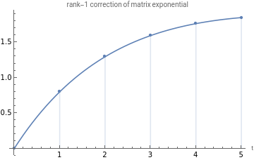
Rank1 correction of matrix exponential
Rank1 correction of matrix exponential
Code
Code
Approximating matrix power with matrix exponential
Approximating matrix power with matrix exponential
In[]:=
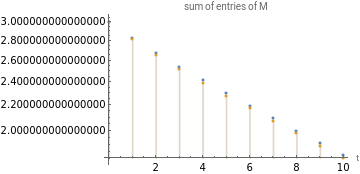
Print[SF["T=``+``",MatrixForm[A],MatrixForm@Hr]];DiscretePlot@@{sum/@{exp[tAsgd],pow[ii+Asgd,t]},{t,0,10},ScalingFunctions->"Log",PlotLegends->{"M=exp(t T)","M=(I+T"},PlotLabel->"sum of entries of M",AxesLabel->{"t"}}
t
)\),
T=
+
- 60 121 | 0 | 0 |
0 | - 48 121 | 0 |
0 | 0 | - 36 121 |
36 121 | 18 121 | 12 121 |
18 121 | 9 121 | 6 121 |
12 121 | 6 121 | 4 121 |
Out[]=
In[]:=
(*" B=",MatrixForm[nf@B]," u=",u];*)init[1];vy=;gSto1y[y_]=;Print["a=",MatrixForm@Diagonal[A]];Print["u=",MatrixForm@u];Print["v(y)=",MatrixForm@vy];Print["f(y)=",gSto1y[y]//FullSimplify];Print["[f](t)=",InverseLaplaceTransform[N@gSto1y[y],y,t]];Print["A=diag(a)=",MatrixForm[A]];Print["B=uu",MatrixForm[B]];trajSto1=InverseLaplaceTransform[gSto1y[y],y,t];plot1=Plot[sum[exp[t(A+B)]-exp[tA]],{t,0,5},PlotLegends->{"<>-<>"},AxesLabel->{"t"}];plot2=DiscretePlot[trajSto1,{t,0,5},PlotLegends->"[f](t)",AxesLabel->{"t"}];Show[plot1,plot2,PlotLabel->"rank-1 correction of matrix exponential"]
u
1-Diagonal[A]/y
1
2
y
1-Dot[vy,u]
-1
y
2
Total[vy]
-1
L
t(A+B)
e
tA
e
-1
L
a=
- 60 121 |
- 48 121 |
- 36 121 |
u=
6 11 |
3 11 |
2 11 |
v(y)=
6 111+ 60 121y |
3 111+ 48 121y |
2 111+ 36 121y |
f(y)=
121
2
(22608+121y(1008+1331y))
(36+121y)(48+121y)(60+121y)(10512+121y(2448+121y(95+121y)))
-1
L
-0.495868t
-0.423048t
-0.396694t
-0.317963t
-0.297521t
-0.0441126t
A=diag(a)=
- 60 121 | 0 | 0 |
0 | - 48 121 | 0 |
0 | 0 | - 36 121 |
B=uu
36 121 | 18 121 | 12 121 |
18 121 | 9 121 | 6 121 |
12 121 | 6 121 | 4 121 |
Out[]=
|