In[]:=
Tue 9 May 2023 00:16:08
Using exp(-At) to approximate (I-A) math.SE post
In[]:=
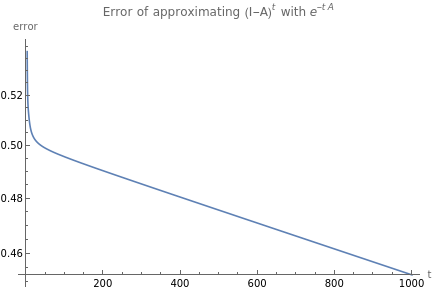
d=10000;maxSteps=1000;p=1.;h=Table[,{i,1,d}];h=h/Max[h];exact[t_]:=Total[];approx[t_]:=Total[Exp[-th]];error[truth_,est_]:=(est-truth);relError[truth_,est_]:=;Print["Tr(A)=",Total[h]]Print["Tr()=",Total[h*h]]ListPlot[h,PlotLabel->"A eigenvalues",ScalingFunctions->{"Log","Log"},Filling->Axis];LogPlot[error[exact[s],approx[s]],{s,1,maxSteps},PlotLabel->"Error of approximating (I-A with ",AxesLabel->{"t","error"}]
-p
i
t
(1-h)
(est-truth)
truth
2
A
t
)\),
-tA
e
Tr(A)=9.78761
Tr()=1.64483
2
A
Out[]=
In[]:=
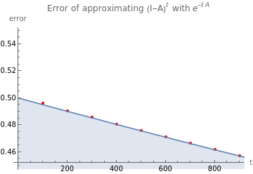
xvals=Table[t,{t,1,maxSteps}];yvals=Table[error[exact[t],approx[t]],{t,xvals}];observedPlot=ListPlot[{xvals,yvals},PlotLegends->{"(t)"}];formula=Exp[-x/d];predictedPlot=Plot[formula,{x,0,d},Filling->Axis,PlotLegends->{formula}];observedPlot=ListPlot[{xvals[[;;;;100]],yvals[[;;;;100]]},PlotStyle->{Red}];Show[observedPlot,predictedPlot,PlotLabel->"Error of approximating (I-A with ",AxesLabel->{"t","error"}]
f
A
1
2
t
)\),
-tA
e
Out[]=
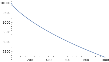
pdf=;int=Inactive[Integrate][pdfExp[-ys],{y,,1}];formulaError=Assuming[{p>=1,d>1,s>1},Activate[int]]
-1/p
(y)
py
-p
(d+1)
Out[]=
In[]:=
errorPlot=Block[{p=1,d=10000},Plot[formulaError,{s,1,maxSteps}]]
Out[]=
Power-Law fits
Power-Law fits
In[]:=
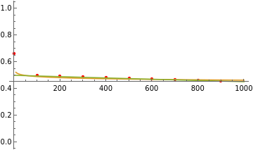
powerLawFit[xvals_,yvals_]:=Module[{logData,linearFit,a,b},logData=Transpose[{Log[xvals],Log[yvals]}];linearFit=LinearModelFit[logData,x,x];{a,b}=linearFit["BestFitParameters"];fit=Exp[a+b*Log[x]];fitModel=Function@@{{x},fit};fitModel];exponentialFit[xvals_,yvals_]:=Module[{logData,linearFit,a,b},logData=Transpose[{xvals,Log[yvals]}];linearFit=LinearModelFit[logData,x,x];{a,b}=linearFit["BestFitParameters"];fit=Exp[a+b*x];fitModel=Function@@{{x},fit};fitModel];f1=powerLawFitxvals;;
d
,yvals;;d
;f2=exponentialFit[xvals[[maxSteps/2;;maxSteps-maxSteps/4]],yvals[[maxSteps/2;;maxSteps-maxSteps/4]]];fittedPlot=Plot[{None,f1[t],f2[t]},{t,0,maxSteps},PlotLegends->{None,f1[t],f2[t]}];Show[observedPlot,fittedPlot,PlotRange->{{0,maxSteps},{0,1}}]Out[]=
In[]:=
f2[x]
Out[]=
-0.692587-0.000100435x