In[]:=
deploy
Tue 6 Sep 2022 11:33:05
In[]:=
d=10000;numSamples=100000;nf[x_]:=NumberForm[x,{5,5}];h=Table[,{i,1,d}];h=h/Total[h];mu=0;gaussianSampler[diag_]:=With{d=Length[diag]},Compile{{n,_Integer}},Module{vals},vals=mu+]];inverseX4=Compile[{{batch,_Real,2}},Module[{x=First@batch},]];PrintStringForm"For d=`` observed=`` predicted=``",nf@d,nf@expectation[inverseX4,1],nf@
-0.5
i
diag
*#&/@RandomVariate[NormalDistribution[],{n,d}];sampler=gaussianSampler[h];(*estimatesaveragevalueoffunconsamplesizes*)expectation[func_,s_]:=With[{numBatches=Max[1,Floor[numSamples/(s*d)]]},Nest[func[sampler@s]+#&,0.,numBatches]/numBatches];Ex4=Total[h]+2Total[h*h];xfourth=Compile[{{batch,_Real,2}},Module[{x=First@batch},2
(x.x)
-2
(x.x)
1
Ex4
For d=10000 observed=0.99667 predicted=0.99950
Average squared dot product in high dimensions?
Average squared dot product in high dimensions?
In[]:=
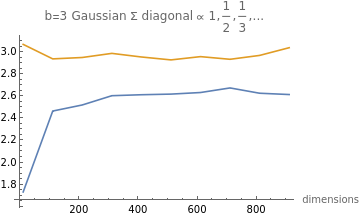
initialize[h0_]:=(d=Length[h0];h=h0;sampler=gaussianSampler[h];sigma=DiagonalMatrix[h];);gaussianSampler[diag_]:=With[{d=Length[diag]},Compile[{{n,_Integer}},Module[{vals},vals=Sqrt[diag]*#&/@RandomVariate[NormalDistribution[],{n,d}]]]];(*estimatesaveragevalueoffunconsamplesizes*)expectation[func_,s_]:=With[{numBatches=Max[1,Floor[Sqrt[s]*numSamples/(s*d)]]},Nest[func[sampler@s]+#&,0.,numBatches]/numBatches];cosineSimilaritySquared=Compile[{{X,_Real,2}},Module[{b=Length[X],meanLengthSquared,X2,gram},meanLengthSquared=Total[Total[#.#]&/@X]/b;X2=#/Norm[#]&/@X;gram=X2.X2;Total@Flatten@(gram*gram)/b/b]];innerProductSquared=Compile[{{X,_Real,2}},Module[{b=Length[X],meanLengthSquared,gram},gram=X.X;Total@Flatten@(gram*gram)/b/b]];getVals[d_,b_]:=(With[{h=Table[i^-1.,{i,1,d}]},initialize[h/Total[h]];];oneOverE=1/expectation[innerProductSquared,b];EoneOver=expectation[1/innerProductSquared[#]&,b];{oneOverE,EoneOver})numSamples=1000000;b=3;dims=Table[d,{d,10,1000,100}];vals=Table[getVals[d,b],{d,dims}];vals=Thread[{dims,#}]&/@{vals[[1]],vals[[2]]};ListLinePlotvals,AxesLabel->{"dimensions"},PlotLegends->{"FractionBox[\(1\), \(E[\(\(<\)\(x\)\), \(\(y\)\*SuperscriptBox[\(>\), \(2\)]\)]\)]","EFractionBox[\(1\), \(\(\(<\)\(x\)\), \(\(y\)\*SuperscriptBox[\(>\), \(2\)]\)\)]"},PlotLabel->StringForm"b=`` Gaussian Σ diagonal ∝ 1,,,...",b
1
2
1
3
Out[]=
Special case b=1 reduces to ||x4||
Special case b=1 reduces to
||x
4
||
In[]:=
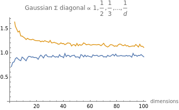
numSamples=100000;(*estimatesaveragevalueoffunconsamplesizes*)expectation[func_,s_]:=With[numBatches=Max[1,,,...,"
s
Floor[numSamples/(s*d)]],Nest[func[sampler@s]+#&,0.,numBatches]numBatches];vals=Table[getVals[d,1],{d,10,1000,10}];ListLinePlotvals,AxesLabel->{"dimensions"},PlotLegends->{"FractionBox[\(1\), \(E[\(||\)\(x\)\*SuperscriptBox[\(||\), \(4\)]]\)]","EFractionBox[\(1\), \(\(||\)\(x\)\*SuperscriptBox[\(||\), \(4\)]\)]"},PlotLabel->"Gaussian Σ diagonal ∝ 1,1
2
1
3
1
d
Out[]=
Is it the case of estimator variance increasing?
Is it the case of estimator variance increasing?
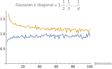
no, same result observed if we scale up the number of samples with dimension
In[]:=
(*scalenumbersampleswithd*)getVals[d_,b_]:=(numSamples=1000*d;With[{h=Table[i^-1.,{i,1,d}]},initialize[h/Total[h]];];oneOverE=1/expectation[innerProductSquared,b];EoneOver=expectation[1/innerProductSquared[#]&,b];{oneOverE,EoneOver});vals=Table[getVals[d,1],{d,10,1000,10}];ListLinePlotvals,AxesLabel->{"dimensions"},PlotLegends->{"FractionBox[\(1\), \(E[\(||\)\(x\)\*SuperscriptBox[\(||\), \(4\)]]\)]","EFractionBox[\(1\), \(\(||\)\(x\)\*SuperscriptBox[\(||\), \(4\)]\)]"},PlotLabel->"Gaussian Σ diagonal ∝ 1,,,...,"
1
2
1
3
1
d
Out[]=