In[]:=
Fri 12 Jul 2024 16:50:53
In[]:=
SF=StringForm;getPowerLaw[yvals_]:=Module[{logData,linearFit,a,b,x,xvals},xvals=Range@Length@yvals;logData=Transpose[{Log[xvals],Log[yvals]}];linearFit=LinearModelFit[logData,x,x];{a,b}=linearFit["BestFitParameters"];fit=Exp[a+b*Log[x]];fitModel=Function@@{{x},fit};fitModel[t]];rowNormalize[dataset_]:=Normalize/@dataset;makeTriangularDataset[d_]:=rowNormalize@LowerTriangularize[ConstantArray[1.,{d,d}]];makeRepeatedDataset[d_]:=IdentityMatrix[d]~Join~IdentityMatrix[d];(*Symmetricsquareroot*)symsqrt[m_]:=Module[{U,S,W},{U,S,W}=SingularValueDecomposition[m];U.Sqrt[S].Transpose[W]];subsample[ll_]:=ll[[;;Min[10,Length@ll],All]];CircleTimes=KroneckerProduct;
Power law fits
Power law fits
Singular values
Singular values
In[]:=
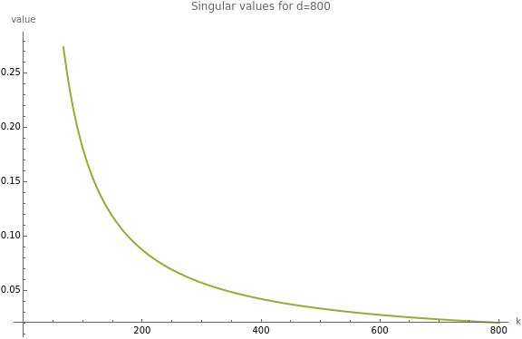
powerLawFit[xvals_,yvals_]:=Module[{logData,linearFit,a,b,x},logData=Transpose[{Log[xvals],Log[yvals]}];linearFit=LinearModelFit[logData,x,x];{a,b}=linearFit["BestFitParameters"];fit=Exp[a+b*Log[x]];fitModel=Function@@{{x},fit};fitModel];rowNormalize[dataset_]:=Normalize/@dataset;svals[d_]:=With[{dataset=rowNormalize@N@UpperTriangularize[ConstantArray[1.,{d,d}]]},SingularValueList[dataset]];d=800;data={Range[d],svals[d]};sf={"Log","Log"};sf={Automatic,Automatic};observedPlot=ListPlot[subsample@data,ScalingFunctions->sf];{xvals,yvals}=data;f=powerLawFit[xvals,yvals]fittedPlot=Plot[{None,None,f[t]},{t,0,Length[xvals]},PlotLegends->{None,None,f[t]},ScalingFunctions->sf];Show[fittedPlot,observedPlot,ImageSize->Large,AxesLabel->{"k","value"},PlotLabel->SF["Singular values for d=``",d]]
Out[]=
Function{x$33105},
21.8692
1.0422
x$33105
Out[]=
Norm as a function of d, Vincent’s plot
Norm as a function of d, Vincent’s plot
In[]:=
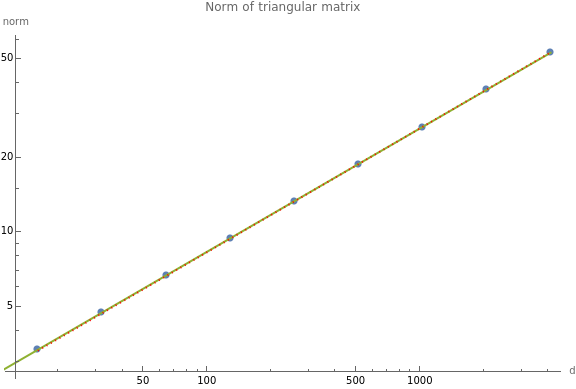
norm[d_]:=With[{dataset=rowNormalize@N@UpperTriangularize[ConstantArray[1.,{d,d}]]},Norm[dataset]];sf={"Log","Log"};(*data=Table[{d,norm[d]},{d,10,1000,10}];*)dimsList=Table[,{k,4,12}];data=Table[{dd,norm[dd]},{dd,dimsList}];observedPlot=ListPlot[subsample@data,ScalingFunctions->sf,PlotLegends->{"empirical"}];{xvals,yvals}=data;f=powerLawFit[xvals,yvals];fittedPlot=Plot[{None,None,f[t]},{t,0,Max[xvals]},PlotLegends->{None,None,f[t]},ScalingFunctions->sf];vincentPlot=Plot
k
2
dLog[2]
,{d,Min[dimsList],Max[dimsList]},ScalingFunctions->sf,PlotStyle->{Red,Thick,Dotted},PlotLegends->SF"vincent dLog[2]
";Show[observedPlot,fittedPlot,vincentPlot,PlotLabel->SF["Norm of triangular matrix",d],ImageSize->Large,AxesLabel->{"d","norm"}]Out[]=
Effective Ranks
Effective Ranks
In[]:=
d=4000;svals=SingularValueList@rowNormalize@N@UpperTriangularize[ConstantArray[1.,{d,d}]];TableForm{"norm",Max[svals]},"R",,"r",svals2=svals/Total[svals];DiscretePlot[Total[],{k,1,100},ScalingFunctions->{Automatic,"Log"},PlotRange->All,PlotLabel->"Singular value moments",AxesLabel->{"k","moment"}]
2
Total[svals]
Total[]
2
svals
Total[svals]
Max[svals]
k
svals2
Eigenvalues and singular values
Eigenvalues and singular values
TLDR:
Eigenvalues fall off exactly as 1/sqrt(d), singular values approximately as 1/d
Right svecs are 0 for the last coordinate
Left svecs are 1 for the last coordinate
Stationary distribution is mostly last coordinate
Eigenvalues fall off exactly as 1/sqrt(d), singular values approximately as 1/d
Right svecs are 0 for the last coordinate
Left svecs are 1 for the last coordinate
Stationary distribution is mostly last coordinate
Comparing density to others
Comparing density to others
Eigenvalues of GD operator
Eigenvalues of GD operator
Choi vs eigenvalues
Choi vs eigenvalues
Do the I-T
Do the I-T