In[]:=
Sat 2 Dec 2023 23:52:40
In[]:=
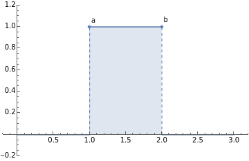
With[{a=1,b=2},points=ListPlot[{Labeled[{a,1},"a"],Labeled[{b,1},"b"]},FillingAxis,FillingStyleDashed];theta=HeavisideTheta[y-a]-HeavisideTheta[y-b];plot=Plot[theta,{y,0,3},Filling->Axis,PlotRangePadding->.2];Show[plot,points]]
Out[]=
In[]:=
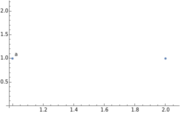
points
Out[]=
In[]:=
g[x_]=;gi=InverseFunction[g];dgi=D[gi[y],y];a=g[0];b=g[∞];theta=HeavisideTheta[y-b]-HeavisideTheta[y-a];
1
2
(1+x)

In[]:=
LaplaceTransform[D[gi[y],y]*y*theta,y,t]//FullSimplify
Out[]=
π
Erf[t
]2
t
In[]:=
Integrate[g[x]Exp[-tg[x]],{x,0,∞}]
Out[]=
π
Erf[t
]2
t
In[]:=
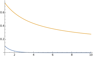
Plot,,{t,1,10}
π
-Erf[t
]+Erf[2
t
]2
t
π
Erf[t
]2
t
Out[]=
Asymptotic
In[]:=
Solve[g[0]==Infinity,x]
Out[]=
{}
In[]:=
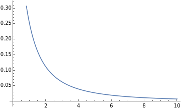
Plot[g[x],{x,0,10}]
Out[]=
In[]:=
g[0]
Out[]=
1
In[]:=
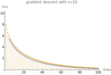
continuousPlot2=Plot[sol2,{s,0,maxStep},PlotRangeAll];Show[discretePlot,continuousPlot2]
Out[]=
In[]:=
IntegrateExp-2s,{i,0,n},Assumptions{n>1,s>1}//FullSimplify
1
2
(i)
Out[]=
-
2s
2
n
2π
s
Erfc2
s
n
In[]:=
Block{n},IntegrateExp-2s,{i,0,nn},Assumptions{nn>1,s>1}
1
2
i
Out[]=
-
2s
2
nn
2π
s
Erfc2
s
nn
In[]:=
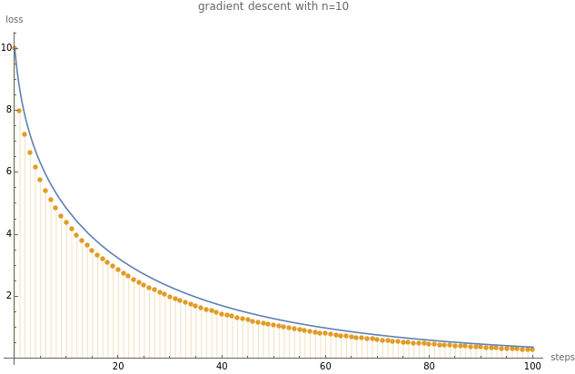
With{nn=10},ShowdiscretePlot,Plotnn-,{s,1,100}
-
2s
2
nn
2π
s
Erfc2
s
nn
Out[]=
In[]:=
LeafCount[-E^-t]
Out[]=
7