This piece is my short attempt at a deeper understanding of some of the most problematic parts of quantum theory concerning quantum computing . Starting from a particular example of the CHSH game, it goes through a diagrammatic representation of quantum theory, non-classical correlations, the emergence of negative probabilities, a multiway version of the Many Worlds interpretation, the nature of qubits, anti-particles, and the role of quantum resources in beyond quantum theories .
Thepathtoquantumenlightenment@SabineHossenfelder
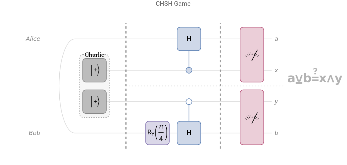
In the CHSH game, there are two cooperating players, Alice and Bob, and a referee, Charlie. At the start of the game, Charlie chooses bits uniformly at random, and then sends to Alice and to Bob. Alice and Bob must then each respond to Charlie with bits respectively. Now, once Alice and Bob send their responses back to Charlie, Charlie tests if . If this equality holds, then Alice and Bob win, and if not then they lose.
x,y∈{0,1}
x
y
a,b∈{0,1}
a⊻b=x∧y
We can easily construct a circuit representing the setup of this game using the Quantum Framework:
PacletInstall["Wolfram/QuantumFramework"]<<Wolfram`QuantumFramework`
Out[]=
Let’s compute the joint probability distribution for all possible outcomes of the experiment:
In[]:=
measurement=chsh[]
Out[]=
QuantumMeasurement


Out[]=
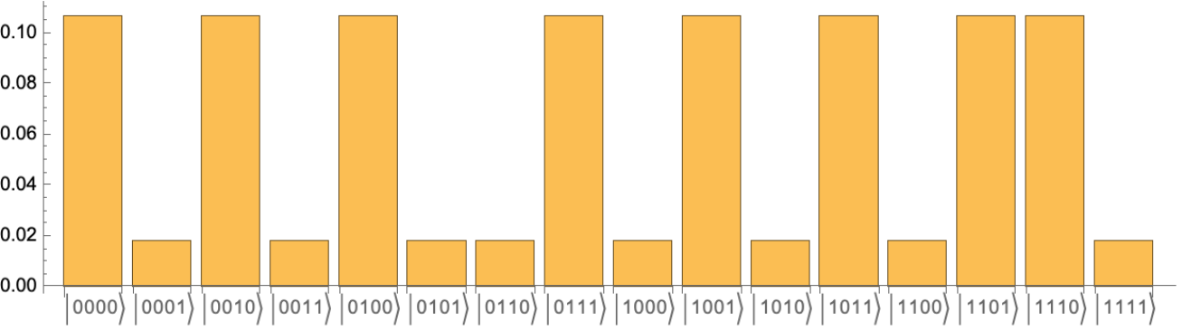
We can also get the underlying multivariate categorical distribution:
In[]:=
distribution=measurement["MultivariateDistribution"]
Out[]=
CategoricalDistribution
Computing probability of winning now is as straight-forward as taking an expectation of the stated criteria :
a⊻b=x∧y
In[]:=
probabilityOfWinning=Simplify@Expectation[Boole[BitXor[a,b]==BitAnd[x,y]],{a,x,y,b}distribution]
Out[]=
1
4
2
)In[]:=
N[probabilityOfWinning]
Out[]=
0.853553
We get a very well known result of achieving ~85% probability of winning using this quantum strategy.
Ok, but what’s the big deal here?
This game is one of the simplest examples of beyond classical correlations (in the Appendix it is shown that no classical strategy can’t reach more than 75% probability of winning at this game).
This game is one of the simplest examples of beyond classical correlations (in the Appendix it is shown that no classical strategy can’t reach more than 75% probability of winning at this game).
It is widely believed that complex numbers are the cause of all the quantum weird behaviour. But actually most of quantum features can just be explained with the right interpretation and classical probability theory (cf. epistricted complementarity, Spekkens toy model, generalize probability theory etc.), but not the case of violating CHSH inequalities and reaching that 85% winning rate in this game.
Imaginary components do not survive until one gets to the actual probability distribution of any real experimental outcome.
So how far one can get with a theory that only operates on probability distributions? Not far enough! And the missing ingredient to get as far as quantum theory are negative probabilities. To which we’ll get later, but first let’s understand how probability distributions differ from quantum states with their complex amplitudes.
Imaginary components do not survive until one gets to the actual probability distribution of any real experimental outcome.
So how far one can get with a theory that only operates on probability distributions? Not far enough! And the missing ingredient to get as far as quantum theory are negative probabilities. To which we’ll get later, but first let’s understand how probability distributions differ from quantum states with their complex amplitudes.
Classical vs Quantum wires
Classical vs Quantum wires
A default wire in the quantum circuit represents a qudit, which in general is a vector of complex amplitudes
Out[]=

In[]:=
ψ=QuantumState["RandomPure"]
Out[]=
(0.0730457-0.627347)|0〉+(0.419035-0.652311)|1〉
The Born rule tells us that in order to get probabilities, state amplitudes should be squared:
In[]:=
ψ["Probability"]
Out[]=
|0〉0.3989,|1〉0.6011
In[]:=
Abs[ψ["Amplitudes"]]^2
Out[]=
|0〉0.3989,|1〉0.6011
Diagrammatically quantum states with amplitudes and classical probability distributions can be represented by a thick and a thin wire respectively:
In[]:=
QuantumCircuitOperator[{"Double"["I"],"I"->2}]
Out[]=
Of course nothing stops one to ‘store’ complex numbers in this thin classical wire too. And that’s what usually happens with the default circuit representation of any quantum computation anyway, like in this simple example:
Out[]=
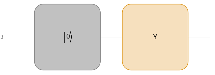
Which just equals to :
|1〉
In[]:=
QuantumCircuitOperator[{"0","Y"}][]
Out[]=
|1〉
But a more natural representation of quantum computation lies in higher dimensions and thick wires.
In the qubit case, thick wire packs four numbers instead of two for every component of underlying density matrix and in qutrits case it would be nine. A general procedure of encoding thin classical probability distribution wire into a quantum thick wire is called doubling (it doubles the amount of wires and squares overall dimensionality).
One can encode a classical probability distribution into its quantum version with a special Encode operator:
In[]:=
QuantumCircuitOperator["Encode"]
Out[]=
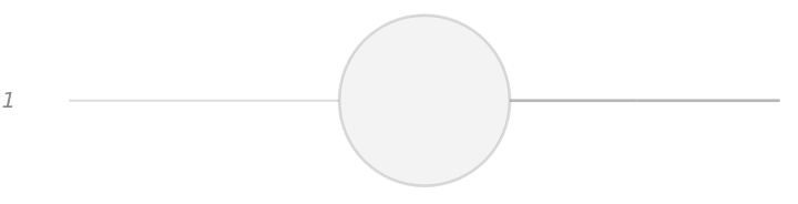
Which just pads a 2-dimensional vector into a 4-dimensional one with zeroes:
QuantumOperator["Encode"]@()
a|0〉+b|1〉
Out[]=
a|0〉+b|3〉
The reverse procedure of thinning the wires is then would naturally represent the idea of measurement, with only these components (the diagonal of a density matrix) being extracted:
In[]:=
QuantumCircuitOperator["Measure"]
Out[]=
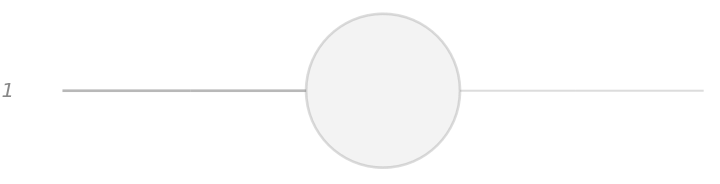
QuantumOperator["Measure"]@()
a|0〉+c|1〉+d|2〉+b|3〉
Out[]=
a|0〉+b|1〉
Quantum circuit can contain wires of different dimensions. While the default thin wire is the usual one representing 2-dimensional qubits classically:
Out[]=
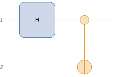
The proper quantum representation would be a thick doubled version of it:
Which is equivalent of having an original circuit with its conjugate version side-by-side and combining their corresponding wires into one:
Having this separation into classical and quantum wires allows us to clearly distinguish probability distributions from general complex density matrices. With this treatment every practical quantum circuit can simultaneously represent both quantum and classical computations together with measurements as a bridge in between, with classical thin wires only carrying real numbers (I’m intentionally not saying real numbers between 0 and 1, because we would still require negative probabilities later).
So what does it mean to measure a qubit?
In its default treatment the Quantum Framework operates classically as much as possible and all the thickening effectively happens under the hood.
Circuit with measurement can be evaluated into a special measurement object, and that’s where all the quantum stuff happens with density matrix being reduced and its diagonal extracted into probabilities:
Circuit with measurement can be evaluated into a special measurement object, and that’s where all the quantum stuff happens with density matrix being reduced and its diagonal extracted into probabilities:
But now we have the tools to bring this onto the surface.
In the Quantum Framework measurements are non-demolishing by default, which means they actually ‘copy’ its input in two:
In other words the measurement operator above is the same as some people call the copy operator (or copy spider):
Let’s do the doubling in a different way, first by adding an initial state and composing it with its adjoint:
This represents now a final density matrix ready for measurement. The second qubit is traced out reducing it to a single qubit matrix:
Tracing diagrammatically is represented by a loop which is itself constructed from a Bell state and its adjoint (because of their shapes also known as a Cup and Cap):
Now the free input wire has to be combined with the output wire to make a thick wire that can be measured:
An easier way of doing the same is to bend these wires around so that there are just two copies of a circuit (original and its conjugate) sitting together side by side:
At this point one can invoke his or her favorite ontology about why an observer only have access to a classical wire output as a probability distribution across ensemble of measurements. For our purposes we just take it as a fact and accept it as a result of specific rules of the universe we live in. But we still can put some more effort into describing and understanding these rules in yet more detail.
Multiway picture of entanglement
Multiway picture of entanglement
Our simple Bell circuit is the simplest example of an entanglement. One can represent its effect as a multiway graph as follows:
Where each individual state is a pure separable state with branching showing superposition explicitly.
Not every two-qubit operator introduces entanglement, for example applying CNOT gate again does not branch anymore:
Not every two-qubit operator introduces entanglement, for example applying CNOT gate again does not branch anymore:
For the doubled case, entanglement now effectively creates a superposition between four separable states (which can’t longer be depicted with a Bloch sphere, so they’re just shown as amplitudes):
In this simple example branching happens with equal probability 1/2 or 1/4 when doubled:
But it’s not hard to construct a circuit with irrational branching probabilities, adding a qubit rotation around Y-axis for example:
If one wishes, it is possible to scale underlying states down and work with unnormalized probability distributions instead. For example these are the first qubits from each branch and their norms:
(Norm has nothing to do with the length of the arrow, length is always equal to sphere radius for pure states)
So instead of tracing probabilities along each path and weighting final states accordingly, the final superposition state can be instead recovered from just the last unnormalized states in the multiway graph by simply summing them over with equal weights:
Branching in a quantum multiway system untangles states making their evolution purely local without any non-local correlations between qubits in each branch.
But is it the case that resulting probability distributions of all classical wires are in fact valid distributions?
But is it the case that resulting probability distributions of all classical wires are in fact valid distributions?
Take the Bell circuit again and its multiway graph:
Two branches result in a weird degenerate distribution with all probabilities equal to zero. But this can interpreted as nothing happening in these branches without affecting the overall joint distribution across all four branches.
These degenerate branches represent off-diagonal elements of the density matrix, and them being zero means there is simply no coherence in this case.
But if there is a coherence like in this case:
Probability distributions in these branches would in general contain not just zero degenerate states, but states with negative probabilities. These will result in destructive interference when states are summed over to make a final superposition state.
How would one reconcile this bizarre notion? Without this negative probability problem, any quantum computation could have been interpreted as a usual multiway system with events acting on underlying probability distributions. When it’s time for a measurement, more events would collect statistical samples across all branches with joint probability arising naturally from the whole process. Any experiment could’ve been repeated multiple times with an observer effectively experiencing a single branch world with different outcomes interpreted as a result of a collective measurement statistics of multiple branches and not just one. While within a single branch, classical probability distributions would have a simple classical explanation of observers being ignorant about reality and performing imperfect measurements, which in turn can also be explained by more branching and observers experiencing their single paths with no correlations between them.
CHSH
CHSH
Before coming up with a solution for negative probabilities, let’s first see how they arise in the CHSH game instead.
The doubled version of the CHSH circuit can be simplified by not doubling Charlie’s part of it as it’s not modified through the computation anyway, and balanced 50/50 amplitudes are the same as 50/50 probabilities.
Out of eight branches in total there are six with negative probabilities.
One can also directly decompose the final joint probability to construct a smaller superposition of separable distributions. Turns out three is enough:
But if one seeks a complete computational approach of everything, branching as a result of applying operators with explicit introduction of entanglement is more natural than going backwards from a final result like this.
One seemingly simple way to make sense of negative probability is to appeal to the fact that within each branch there exists a basis in which probability distribution is very simple:
But what is a basis of the classical probability distribution? Why would there be linear combinations of coin toss outcomes like (1/2 tails - 1/4 heads)? What does it mean for there to be X amount of 60/40 mixture of winning and losing within one particular branch? Well, it doesn’t really matter as it just making things worse by allowing not just negative outcomes, but arbitrary linear combinations of them and then assigning them a positive probability.
No matter how hard one tries there has to be model for negative outcomes, outcomes with negative probability.
Negative outcomes
Negative outcomes
It is very tempting to bring the idea of anti-particles and particle anti-particle annihilation into the picture and explain everything by them somehow. This analogy though requires very careful treatment, especially when negative outcomes combine into a joint distribution.
So why not, similar to how doubling of a classical wire and consequent measuring helps us to get rid off imaginary components, introduce a different kind of doubling where each outcome would have a negative counterpart effectively squaring overall dimension once more.
And in fact, because qubits do not exist in nature as elementary constituents due to their inherent fermionic vector structure with local bosonic tensor product structure. Qubit only exists at least as a pair of fermion or boson particles, it is always composite, a Cooper pair, quantum dot or even a whole Rubidium atom. Therefore interpreting each qubit as a pair of particles makes this model even more and not less physical.
In our particular case of eight CHSH branches there are in total 59 non-zero probability outcomes after introducing negative ones (represented by red here):
And as a final joint superposition:
When doing quantum statistics introduction of complex amplitudes is justified by the fact that we can’t explain the results of the experiments with locally evolving probability distributions. But this ‘negative outcome doubling’ procedure restores locality to the picture of evolving PDFs. Evolution is local in space that is, but not in branchial space.
One way to completely get rid of imaginary amplitudes as part of underlying physical states is to work in phase space instead.
Wigner basis and phase space
Wigner basis and phase space
When negative probabilities are involved some people would immediately be reminded of quasi-probability distributions, Wigner functions and phase space representations of quantum states. So what are those?
It’s really all about basis conversion. There is a special basis, called Wigner basis, that can be defined for any dimension:
One can convert any state or operator into this basis using QuantumWignerTransform function:
Also notice that the dimension of a state is a square of the original dimension. And indeed it is equivalent to converting a doubled state into Wigner basis of the same dimension:
The reverse of Wigner transform can be computed using QuantumWeylTransform:
Operators can also be converted to the Phase Space picture, and their action on states is preserved:
This is a discrete phase space representation of a random mixed state:
Or at least it’s that simple for odd dimensions (or integer spin).
For even dimensional (or half-integer spin) qudits, phase space can be split into four independent regions with sign changing when some of them wrap around, that’s why it is not very natural:
Fourier operators therefore can be thought of as square roots of reflection in phase space!
Note that higher dimensional operators acting on qudits are not the same as stacking single-qubit operators together to form multi-qubit systems like this:
Which would introduce external coordinate space degree of freedom, formed by the tensor product, in addition to the internal ones of each qudit.
This observation makes one wonder whether qubits are the sole reason for why quantum computation in phase space is not so widely adopted.
But now at least we can imagine a quantum computation model that only deals with usual probability distributions being modified in a conventional multiway fashion, no different than any classical computation described in similar way.
Beyond quantum correlations
Beyond quantum correlations
As a final note, let’s explore what happens to our CHSH example when one doubles once more.
With another double procedure, our strategy can get us to ~97% probability of winning! But are these circuits realizable in real life?
The only problematic part in this setup is this spider:
Which essentially turns two quantum wires into one or equivalently one super-quantum wire into a single quantum one or two classical ones.
Note that this spider is not a quantum spider itself, because it’s not the doubled classical spider, but both are confusingly represented by the same diagram:
Doubled spider could’ve been constructed (up-to a phase) from a GHZ state and post-selection Caps (what post-selection means will be shown explicitly later):
From classical to quantum analogy this spider performs super-quantum measurement by extracting only diagonal elements of “super-quantum density matrix”.
Even though super-quantum measurement maybe not realizable directly, we actually have a usual quantum measurement after. Composition of those can be realized with non-demolishing measurement of one qubit + post-selection Cap:
Let’s bring it all together:
And let’s also turn Bob’s rotation gates into a single RY(π/2) while we are at it:
This strategy now achieves a perfect score of 100% winning rate (or 97% with the old rotations)!
So are we cheating here or not? Well, yes and no. Post-selection that is done by Alice and Bob allows them to essentially tell Charlie-the-referee to only count certain games and not all of them. But if we allow for a slight relaxation of rules, allowing participants to not answer at all or pretend that their equipment is broken or something, then they can win every single time that actually counts!
This can potentially be interpreted as direct harvesting of quantum resources to achieve statistical advantage.
This can potentially be interpreted as direct harvesting of quantum resources to achieve statistical advantage.
What does post-selection mean in this case exactly? It just means the output quantum wire carries the post-measurement (collapsed) quantum state now and we can use it to entangle with the second Bell pair’s qubit and check whether they produce the same result after a classical measurement. In other words the circuit above is equivalent to this one:
Let’s make a classical version of it with measurements and do a post-selection explicitly:
Post-selection discards every losing outcome and sometimes even discards winning outcomes too, like 1001 or 1110 (discarded outcomes shown in red):
So even though we have a very trivial uniform joint distribution at the end, information gathered using an addition Bell pair allows Alice and Bob to chose only the winning states independently from each other:
What happens if we keep doubling, adding more and more quantum resources in possession of Alice and Bob?
Even without changing Bob’s rotation strategy, the result is almost perfect, achieving 99.9999% probability of winning:
And again we can ask what is this another spider measurement cascade now?
We can analogously turn it into a post-selection as before and also realize it experimentally:
The fact that this doubling procedure systematically increases winning chances suggests that it is a general naive procedure for turning entanglement resource into information. And no optimization over possible operations is required, as for the case of slight change to Bob’s rotations which can already achieve 100% with just a single doubling.
Appendix
Appendix
CITE THIS NOTEBOOK
CITE THIS NOTEBOOK
On quantum amplitudes, correlations and negativity
by Nikolay Murzin
Wolfram Community, STAFF PICKS, October 3, 2023
https://community.wolfram.com/groups/-/m/t/3026423
by Nikolay Murzin
Wolfram Community, STAFF PICKS, October 3, 2023
https://community.wolfram.com/groups/-/m/t/3026423