1011 / Sin / Sinc
1011 / Sin / Sinc
In[]:=
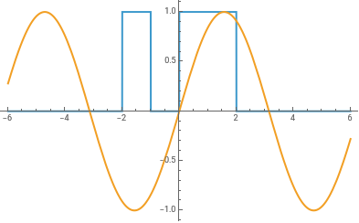
piecewise=Piecewise[{{0,#<-2},{1,#<-1},{0,#<0},{1,#<2}}]&;
In[]:=
Plot[{piecewise[x],Sin[x]},{x,-6,6},Exclusions->None]
Out[]=
In[]:=
SeedRandom[23049829048];trainingx=RandomReal[{-3,3},5000];
In[]:=
trainingy=piecewise/@trainingx;
In[]:=
trainingySin=Sin/@trainingx;
In[]:=
SeedRandom[40985093850948];trainingxSinc=RandomReal[{-32,32},5000];
In[]:=
trainingySinc=Sinc/@trainingxSinc;
In[]:=
ClearAll[TrainPiecewise];TrainPiecewise[net_,x_,y_,seed_Integer:182731,opts___]:=Module[{res,checkpoints={},initNet},initNet=NetInitialize[net,RandomSeeding->seed];res=NetTrain[initNet,x->y,All,opts,TrainingProgressFunction{Function[AppendTo[checkpoints,#Net];],"Interval"Quantity[10,"Rounds"]},MaxTrainingRounds->15000,BatchSize->5000];{res,Prepend[checkpoints,initNet]}]
In[]:=
RRnet[lws_List,activationFn_:Ramp,opts___]:=NetChain[Join[Riffle[LinearLayer/@lws,activationFn],{activationFn,LinearLayer[]}],"Input"->"Real","Output"->"Real"]
1011
1011
In[]:=
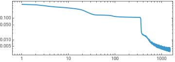
experiment=TrainPiecewise[RRnet[{5,5,5,5}],trainingx,trainingy,182731,TargetDevice->"GPU"];
In[]:=
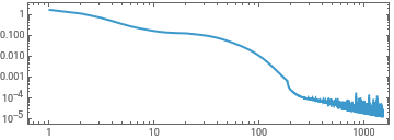
ListLinePlot[First[experiment]["RoundLossList"][[;;;;10]],ScalingFunctions->{"Log","Log"},Frame->True,AspectRatio->1/3]
Out[]=
In[]:=
With[{net=experiment[[-1,-10]]},ListLinePlot[Table[net[x],{x,-3,3,1/16}]]]
Out[]=
In[]:=
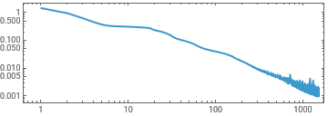
experiment2=TrainPiecewise[RRnet[{8,8,8}],trainingx,trainingy,TargetDevice->"GPU"];
In[]:=
ListLinePlot[First[experiment2]["RoundLossList"][[;;;;10]],ScalingFunctions->{"Log","Log"},Frame->True,AspectRatio->1/3]
Out[]=
In[]:=
With[{net=experiment2[[-1,-1]]},ListLinePlot[Table[net[x],{x,-3,3,1/16}]]]
Out[]=
Sin[x]
Sin[x]
In[]:=
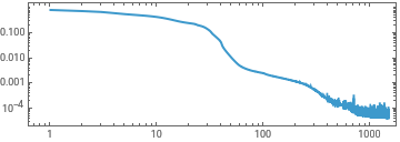
experimentSin=TrainPiecewise[RRnet[{5,5,5,5}],trainingx,trainingySin,TargetDevice->"GPU"];
In[]:=
ListLinePlot[First[experimentSin]["RoundLossList"][[;;;;10]],ScalingFunctions->{"Log","Log"},Frame->True,AspectRatio->1/3]
Out[]=
In[]:=
With[{net=experimentSin[[-1,-1]]},ListLinePlot[Table[net[x],{x,-3,3,1/16}]]]
Out[]=
In[]:=
experimentSin2=TrainPiecewise[RRnet[{8,8,8}],trainingx,trainingySin,TargetDevice->"GPU"];
In[]:=
ListLinePlot[First[experimentSin2]["RoundLossList"][[;;;;10]],ScalingFunctions->{"Log","Log"},Frame->True,AspectRatio->1/3]
Out[]=
In[]:=
With[{net=experimentSin2[[-1,-1]]},ListLinePlot[Table[net[x],{x,-3,3,1/128}]]]
Sinc[x]
Sinc[x]
“Should also make this plot normalizing by total norm of the weights....”
“Should also make this plot normalizing by total norm of the weights....”
GZip complexity
GZip complexity
Networks become less compressible throughout training, indicating an increase in information content.
WeightGzipComplexity[] - Compression ratio of weights serialized as Real64 then gzipped. Lower = more compressible = more structure.
Weight histograms
Weight histograms
3D surface of weight value histograms over training.
X-axis: weight value, Y-axis: checkpoint, Z-axis: bin count.
X-axis: weight value, Y-axis: checkpoint, Z-axis: bin count.
Density plot of all weight values (all layers combined) over training.
X-axis: weight value, Y-axis: checkpoint, colour: bin count.
X-axis: weight value, Y-axis: checkpoint, colour: bin count.
Density plot of weight value distributions per layer over training.
X-axis: weight value, Y-axis: checkpoint, colour: bin count.
X-axis: weight value, Y-axis: checkpoint, colour: bin count.
Claim: as training progresses the rank of the weight matrices decreases (?)
Claim: as training progresses the rank of the weight matrices decreases (?)
Heat map of singular value magnitudes per layer over training. X-axis: SV index, Y-axis: checkpoint, colour: magnitude.
Effective rank via exponential entropy of normalized singular values. 1 = all energy in one SV, n = energy spread equally across n SVs.
MNIST (a more “information dense” problem)
MNIST (a more “information dense” problem)
Loss / Error curves
Loss / Error curves
Effective Rank
Effective Rank
Weight density
Weight density
GZip complexity
GZip complexity
Correlations
Correlations
“Microscopically, we could study correlations between weight values... (e.g. how correlated are the weights across the network; could be that correlations are exponentially damped.... or maybe not)”
Weight change correlation vs layer distance over training.
For each checkpoint, computes how each layer’s weights changed from initialization (ΔW).
For each pair of layers, correlates the QQ-aligned magnitude distributions of their ΔW.
Plots mean correlation as a function of layer distance (x) and checkpoint (y).
Tests whether co-adaptation between layers decays with depth separation.