What generic regularities exist in trained vs. untrained networks?
What generic regularities exist in trained vs. untrained networks?
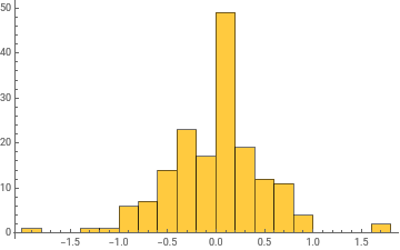
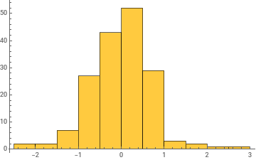
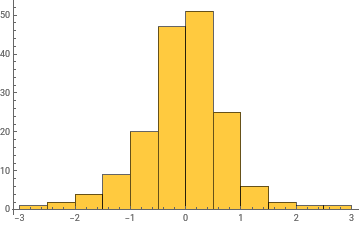
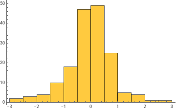
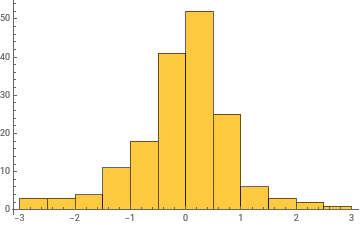
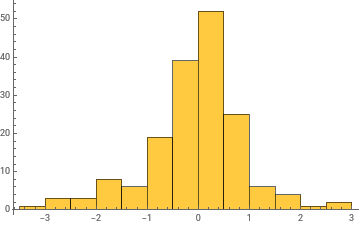
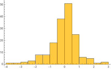
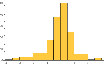
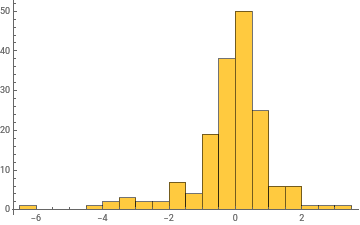
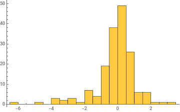
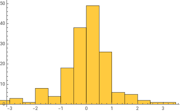
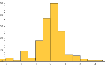
What is the initialized distribution? Generally, the tails of the weight distribution get longer during training...
In[]:=
piecewise=Piecewise[{{0,#<-2},{1,#<-1},{0,#<0},{1,#<2}}]&;SeedRandom[23049829048];trainingx=RandomReal[{-3,3},5000];trainingy=piecewise/@trainingx;
In[]:=
(*===TrainingFunction===*)TrainPiecewise[net_,seed_Integer]:=Module[{res,checkpoints={},initialNet},initialNet=NetInitialize[net,RandomSeeding->seed];res=NetTrain[initialNet,trainingx->trainingy,All,TrainingProgressFunction->{(AppendTo[checkpoints,#Net]&),"Interval"->Quantity[10,"Rounds"]},MaxTrainingRounds->15000,BatchSize->5000,RandomSeeding->seed];{res,Prepend[checkpoints,initialNet]}]
In[]:=
numInstances=5;architecture={8,8,8};
In[]:=
RRnet[lws_List]:=NetChain[Join[Riffle[LinearLayer/@lws,Ramp],{Ramp,LinearLayer[]}],"Input"->"Real","Output"->"Real"]
In[]:=
allResults=Table[(Echo["Training instance ",i];TrainPiecewise[RRnet[architecture],123456*i]),{i,numInstances}];
»
1Training instance
»
2Training instance
»
3Training instance
»
4Training instance
»
5Training instance
In[]:=
allResults
Out[]=
$Aborted
In[]:=
allCheckpoints=allResults[[All,2]];FlattenWeights[net_]:=Join@@Table[With[{layer=NetExtract[net,i]},If[Head[layer]===LinearLayer,Join[Flatten[Normal[NetExtract[layer,"Weights"]]],Flatten[Normal[NetExtract[layer,"Biases"]]]],{}]],{i,Length[net]}]allWeights=Map[FlattenWeights,allCheckpoints,{2}];Print["Weight dimensions: ",Dimensions[allWeights]];allWeightsFlat=Flatten[allWeights,1];
Weight dimensions: {5,1501,169}
In[]:=
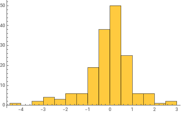
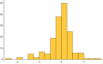
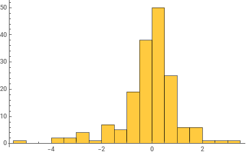
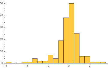
Histogram/@Take[allWeights[[1]],{1,-1,100}]
Out[]=
,
,
,
,
,
,
,
,
,
,
,
,
,
,
,
In[]:=
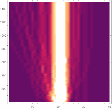
ListDensityPlot[BinCounts[#,{-5,5,.25}]&/@allWeights[[1]]]
Out[]=
In[]:=
ListPlot3D[BinCounts[#,{-5,5,.25}]&/@allWeights[[1]]]
Out[]=

In[]:=
ListPlot3D[BinCounts[#,{-5,5,.25}]&/@allWeights[[1]],PlotRange->All,ScalingFunctions->{Identity,Identity,"Log"}]
Out[]=

In[]:=
ListLinePlot[Variance/@allWeights[[1]]]
Out[]=
In[]:=
ListLinePlot[(Variance/@#)&/@allWeights]
Out[]=
General claim: as the network trains, the distribution of weight values broadens
General claim: as the network trains, the distribution of weight values broadens
Microscopically, we could study correlations between weight values... (e.g. how correlated are the weights across the network; could be that correlations are exponentially damped.... or maybe not)
Can look at this as a function of network depth...
More ...
More ...
Investigations
Investigations
Look at MLPs of different widths and depths
Look at larger single networks, vs. ensembles of networks
◼
Distribution of all weights as a function of training
◼
Distribution of weights per layer as a function of training
We also want to look at individual weights vs. training rounds.....
Should also make this plot normalizing by total norm of the weights....
Take grid networks... Can one visually see training?
◼
How do these results change if one changes the target function?
Richard observes that adversarially changing a few weights won’t affect results, usually....
Claim: as training progresses the rank of the weight matrices decreases (?)
Claim: as training progresses the rank of the weight matrices decreases (?)