Causal Foliations and Causal Cones
Causal Foliations and Causal Cones
We have discussed causal invariance in terms of path independence in multiway systems. But we can also explore it in terms of specific evolution histories for the underlying substitution system. Consider the rule {BAAB}. Here is a representation of one way it can act on a particular initial string:
Out[]=
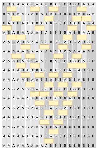
In a multiway system, each path represents a particular sequence of updates that occur one after another. But here in showing the action of {BAAB} we are choosing to draw several updates on the same row. If we want, we can think of these updates as being done in sequence, but since they are all independent, it is consistent to show them as we do.
If we annotate the picture by showing causal connections between updates, we see the causal graph for the evolution---and we see that the updates we have drawn on the same row are indeed independent: they are not connected in the causal graph:
If we annotate the picture by showing causal connections between updates, we see the causal graph for the evolution---and we see that the updates we have drawn on the same row are indeed independent: they are not connected in the causal graph:
In[]:=
SubstitutionSystemCausalPlot[evo,EventLabelsFalse,CellLabelsTrue,CausalGraphTrue]
Out[]=

The picture above in effect uses a particular updating order. The pictures below show three possible random choices of updating orders. In each case, the final result of the evolution is the same. The intermediate steps, however, are different. But because our rule is causal invariant, the causal graph of causal relationships always has exactly the same form:
In[]:=
SeedRandom[242444];GraphicsRow[Table[SubstitutionSystemCausalPlot[SubstitutionSystemCausalEvolution[{"BA"->"AB"},"BBAAAABAABBABBBBBAAA",15,{"Random",4}],EventLabelsFalse,CellLabelsTrue,CausalGraphTrue],3],ImageSizeFull]
Out[]=

In picking updating orders there is always one constraint: no update can happen until the input for it is ready. In other words, if the input for update V comes from the output of update U, then U must already have happened before V can be done. But so long as this constraint is satisfied, we can pick whatever order of updates we want.
It is sometimes convenient, however, to think in terms of “complete steps of evolution” in which all updates that could yet be done have been done. And for the particular rule we are currently discussing, we can readily do this, separating each “complete step” in the pictures below with a dotted line:
It is sometimes convenient, however, to think in terms of “complete steps of evolution” in which all updates that could yet be done have been done. And for the particular rule we are currently discussing, we can readily do this, separating each “complete step” in the pictures below with a dotted line:
In[]:=
With[{evoSequential=SubstitutionSystemCausalEvolution[{"BA"->"AB"},"BBAAAABAABBABBBBBAAA",12]},SubstitutionSystemCausalPlot[evo,EventLabelsFalse,CellLabelsTrue,CausalGraphTrue,PlotSpaceSurfaces((FoldList[Join[#,#2]&,{},TakeList[Range[Total[#]],#]&@(Length/@Rest[evoSequential]〚All,2〛)])/.(FindGraphIsomorphism@@causalGraph/@elementTransitionGraph/@{evoSequential,evo})〚1〛)]]
Out[]=
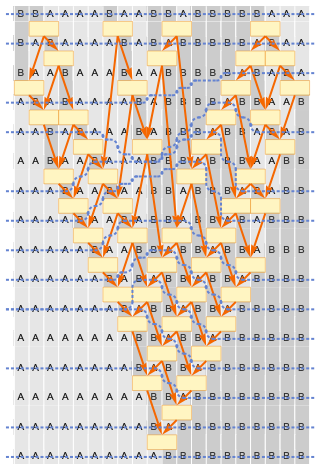
Where the dotted lines go depends on the update order we choose. But because of causal invariance it is always possible to draw them to delineate steps in which a collection of independent updates occur.
Each choice of how to assign updates to steps in effect defines a foliation of the evolution. We will call foliations in which the updates at each step are causally independent "causal foliations". Such causal foliations are in effect orthogonal to the connections defined by the causal graph. (In physics, the analogy is that the causal foliations are like foliations of spacetime defined by a sequence of spacelike hypersurfaces, with connections in the causal graph being timelike.)
The fact that our underlying substitutions (in this case just BAAB) involve neighboring elements implies a certain locality to the process of evolution. The consequence of this is that we can meaningfully discuss the "spatial" spreading of causal effects. For example, we imagine changing (we are not changing anything here) one event in our system, and then seeing what other events can be affected by this:
In[]:=
SubstitutionSystemCausalPlot[evo,EventLabelsFalse,CellLabelsTrue,CausalGraphTrue,CausalConeTrue,CausalConeRoot3]
Out[]=
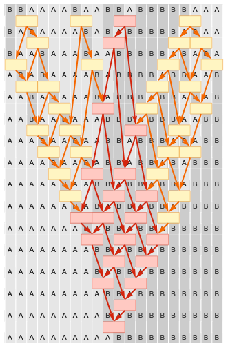
In effect there is a cone (here just two-dimensional) of elements in the system that can be affected. We will call this the causal cone for the evolution. (In physics, the analogy is a light cone.) If we pick a different updating order, the causal cone is distorted. But viewed in terms of the causal foliations, it is exactly the same:
In[]:=
SeedRandom[12820];With[{evo=SubstitutionSystemCausalEvolution[{"BA"->"AB"},"BBAAAABAABBABBBBBAAA",16,{"Random",4}]},SubstitutionSystemCausalPlot[evo,EventLabelsFalse,CellLabelsTrue,CausalGraphTrue,CausalConeTrue,CausalConeRoot3]]
Out[]=

We can also look at this in terms of the causal graph. Each node in the causal graph corresponds to an event. And if we change one event, the connections in the causal graph define what other events can be affected. The result is a rendering of the causal cone inside the causal graph:
Now let us turn things around. Imagine we have a causal graph. Then we can ask how it relates to an actual sequence of states generated by a particular path of evolution. The picture below shows how we can arrange a causal graph so that its nodes---corresponding to events---appear in an order that follows a particular path of evolution:
But the intrinsic structure of the causal graph defines a way to arrange it in layers. And these layers correspond precisely to the causal foliation:
The rule BAAB that we are using here has many simplifying features. But the concepts of causal foliations and causal cones are general, and will be important in much of what follows.
At it happens, we have already implicitly seen both ideas. The "standard updating order" for our main models defines a foliation (similar, in fact, to the first one we showed here (the first one is random), in which in some sense "as much gets done as possible" at each step)---though the foliation is only a causal one if the rule used is causal invariant.
In addition, on page XXXX we discussed how the effect that a small change in the state in one of our models can spread on subsequent steps, and this is just like the causal cone we are discussing here.
Causal Graphs for Infinite Evolutions
Causal Graphs for Infinite Evolutions
One of the simplifying features of the rule BAAB discussed in the previous subsection is that for any finite initial condition, it always evolves to a definite final state after a finite number of steps---so it is possible to construct a complete multiway causal graph for it, and for example to verify that all the causal graphs for specific paths of evolution are identical.
But consider the rule {ABB,BA}:
But consider the rule {ABB,BA}:
This rule is causal invariant, but never evolves to a definite state, and instead keeps growing forever. Including events in the evolution we get:
The corresponding multiway causal graph is:
And now if we extract possible individual causal graphs from this, we get:
These look somewhat similar, they are not directly equivalent. And the reason for this has to do with how we are “counting steps” in the evolution of our system. If we evolve for longer, the effect becomes progressively less important. Here are causal graphs generated by a few different randomly chosen specific sequences of updates (each corresponding to a specific path through the multiway system):
Here are the corresponding results after a few more updates:
This is a different rendering:
And this is what happens after many more updates (with a somewhat more systematic ordering):
If we continued for an infinite number of updates, all these would give the same result---and the same infinite causal graph, just as we expect from expect from causal invariance. But in the particular cases we are showing, they are being cut off in different ways. And this is directly related to the causal foliations we discussed in the previous subsection.
Here are examples of evolution with several specific choices of updating orders:
Here are examples of evolution with several specific choices of updating orders:
Here is what happens if we continue these for longer:
If we now include the causal graphs we can see that they at least start out the same:
Causal graphs on such small plots are unreadable, besides different layout makes it very hard to see they are the same, so I plotted the causal graphs separately. Also, it is easy to see from these causal graphs that they are the same, just cut differently on the bottom, so maybe we should just draw horizontal lines across the plots above, and not have the next picture at all?
But when we also include the causal foliation we see why the causal graphs end differently: each particular path of evolution cuts off the causal graph differently:
XXXXX
But if we were to look just at a specific number of complete steps in the causal foliation, then we would see the exact same causal graph in each case.
XXXXX
But if we were to look just at a specific number of complete steps in the causal foliation, then we would see the exact same causal graph in each case.
[[[[[[[ Start at any point in causal graph; causal cone defines a definite foliation ]]]]]]