In[]:=
ResourceFunction["MultiwaySystem"][CellularAutomaton[90],{{0,0,0,1,0,0,0}},4]
Out[]=

In[]:=
ResourceFunction["MultiwaySystem"][CellularAutomaton[90],{{0,0,1,0,0}},2,"StatesGraph",VertexSize1,PerformanceGoal"Quality"]//LayeredGraphPlot
Out[]=

In[]:=
ResourceFunction["MultiwaySystem"][CellularAutomaton[90],{{0,0,1,0,0}},6,"StatesGraph",VertexSize2]//LayeredGraphPlot
Out[]=

In[]:=
ResourceFunction["MultiwaySystem"][CellularAutomaton[90],{{0,0,0,1,0,0,0}},6,"StatesGraph",VertexSize2]//LayeredGraphPlot
Out[]=

In[]:=
Thread[Tuples[{1,0},3]->IntegerDigits[30,2,8]]
Out[]=
{{1,1,1}0,{1,1,0}0,{1,0,1}0,{1,0,0}1,{0,1,1}1,{0,1,0}1,{0,0,1}1,{0,0,0}0}
In[]:=
ResourceFunction["SequentialCellularAutomaton"][0,3][{1,1,1,1,1}]
Out[]=
{1,1,0,1,1}
Is there any updating order that gives the same result as the ordinary CA?
Is there any updating order that gives the same result as the ordinary CA?
In[]:=
ArrayPlot[Downsample[ResourceFunction["SequentialCellularAutomaton"][90,CenterArray[{1},20],Flatten[Table[Range[20],50]]],{20,1}]]
Out[]=
In[]:=
CloudGet["https://wolfr.am/KXgcRNRJ"];ArrayPlot[CellularAutomaton[30,{{1},0},15],ColorRules{0White,1Black},FrameNone,Epilog{Lighter[Red,.3],Thick,Table[Line[arrayPlotFoliationLine[k,15]],{k,1,47,3}]}]
Out[]=

In[]:=
CloudGet["https://wolfr.am/KXgcRNRJ"];ArrayPlot[CellularAutomaton[30,{{1},0},5],ColorRules{0White,1Black},FrameNone,Epilog{Lighter[Red,.3],Thick,Table[Line[arrayPlotFoliationLine[k,5]],{k,1,17,3}]}]
Out[]=
CA “bricks” are easier to understand....
CA “bricks” are easier to understand....
CellularAutomaton
In[]:=
brules={{{2,2}{2,2},{1,1}{1,1},{1,2}{1,2},{2,1}{2,1},{2,0}{2,0},{1,0}{0,1},{0,2}{0,2},{0,1}{1,0},{0,0}{0,0}},{{2,2}{1,1},{1,1}{2,2},{1,2}{2,1},{2,1}{1,2},{2,0}{0,2},{1,0}{1,0},{0,2}{2,0},{0,1}{0,1},{0,0}{0,0}},{{2,2}{1,1},{1,1}{2,2},{1,2}{1,2},{2,1}{2,1},{2,0}{0,2},{1,0}{1,0},{0,2}{2,0},{0,1}{0,1},{0,0}{0,0}},{{2,2}{2,2},{1,1}{1,1},{1,2}{1,2},{2,1}{2,1},{2,0}{1,0},{1,0}{0,2},{0,2}{0,1},{0,1}{2,0},{0,0}{0,0}}};
In[]:=
brules[[3]]
Out[]=
{{2,2}{1,1},{1,1}{2,2},{1,2}{1,2},{2,1}{2,1},{2,0}{0,2},{1,0}{1,0},{0,2}{2,0},{0,1}{0,1},{0,0}{0,0}}
In[]:=
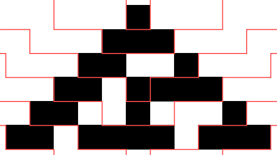
ArrayPlot[BlockCellularAutomaton[brules[[3]],CenterArray[Table[2,38],100],200,1]]
Out[]=

Size 3 block rules
Size 3 block rules
The importance of foliations .... [[ With a different foliation, this gives the R30 pattern ]]
The importance of foliations .... [[ With a different foliation, this gives the R30 pattern ]]
The weird behavior is because we have blocks based on wraparound....
“Approximation lengths”
“Approximation lengths”
Quiescent instead of wraparound
Quiescent instead of wraparound
Which rules show causal invariance?
Which rules show causal invariance?