In[]:=
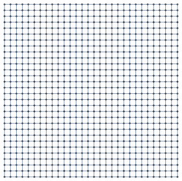
GridGraph[{30,30}]
Out[]=
In[]:=
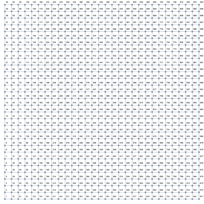
GridGraph[{30,30},VertexLabelsAutomatic]
Out[]=
In[]:=
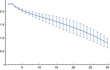
HypergraphDimensionEstimateList[List@@@EdgeList[%]]
Out[]=

In[]:=
ListLinePlot[%]
Out[]=
In[]:=
CenteredDimensionEstimateList
,GraphCenter

Out[]=
{2.32193,2.35658,2.27309,2.21694,2.17913,2.15229,2.13236,2.11699,2.1048,2.0949,2.08671,2.07981,2.07392,2.06884,1.99986,1.82378,1.62282,1.45375,1.30614,1.17319,1.05022,0.933832,0.821433,0.710955,0.600658,0.488999,0.374539,0.255868,0.131537,0.0339047}
In[]:=
ListLinePlot[%]
Out[]=
Corner:
In[]:=
ListLinePlotCenteredDimensionEstimateList
,{900}
Out[]=
In[]:=
GraphNeighborhoodVolumes
,{900},Automatic
Out[]=
900{1,3,6,10,15,21,28,36,45,55,66,78,91,105,120,136,153,171,190,210,231,253,276,300,325,351,378,406,435,465,494,522,549,575,600,624,647,669,690,710,729,747,764,780,795,809,822,834,845,855,864,872,879,885,890,894,897,899,900}
In[]:=
GraphNeighborhoodVolumes
,GraphCenter
,Automatic
Out[]=

In[]:=
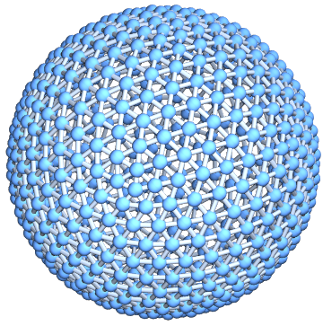
MeshConnectivityGraph[DiscretizeGraphics[Sphere[]]]
Out[]=
Gauss-Bonnet
Gauss-Bonnet
Integrate Gaussian curvature over surface
Sphere
Sphere
Hyperboloid
Hyperboloid