In[]:=
DirectedGraph[Flatten[Table[{v[{i,j}]v[{i+1,j}],v[{i,j}]v[{i+1,j+1}]},{i,10},{j,i}]],VertexCoordinatesCatenate[Table[v[{i,j}]({2(#2-#1/2),-#1}&@@{i,j}),{i,11},{j,i}]],VertexLabelsAutomatic,AspectRatioAutomatic]
Out[]=

In[]:=
regularCausalGraphPlot[layerCount_:9,lineDensity_:1,tan_:0.3,transform_:(#&)]:=DirectedGraph[Flatten[Table[{v[{i,j}]v[{i+1,j}],v[{i,j}]v[{i+1,j+1}]},{i,layerCount-1},{j,i}]],VertexCoordinatesCatenate[Table[v[{i,j}]transform[{2(#2-#1/2),-#1}&@@{i,j}],{i,11},{j,i}]],VertexLabels{x_Placed[Row[Riffle[First[x],","]],Center]},VertexSize.33,VertexStyleLightYellow,AspectRatioAutomatic,Epilog{Style[Table[Line[transform/@{{-100,k-100tan},{100,k+100tan}}],{k,-100.5,100.5,1/lineDensity}],Red]}]
In[]:=
ArcTan[1.]/°
Out[]=
45.
In[]:=
regularCausalGraphPlot[10,1,0,lorentz[0.]]
Out[]=
In[]:=
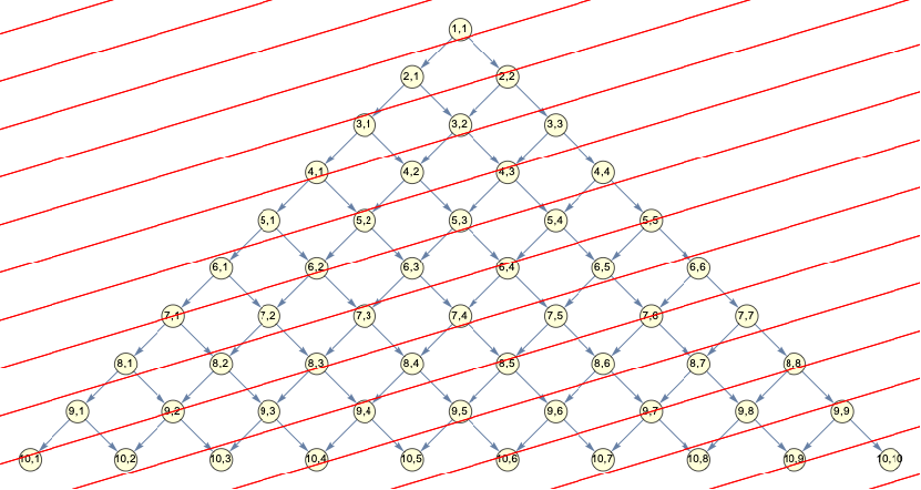
regularCausalGraphPlot[10,1,0.3,lorentz[0.]]
Out[]=
In[]:=
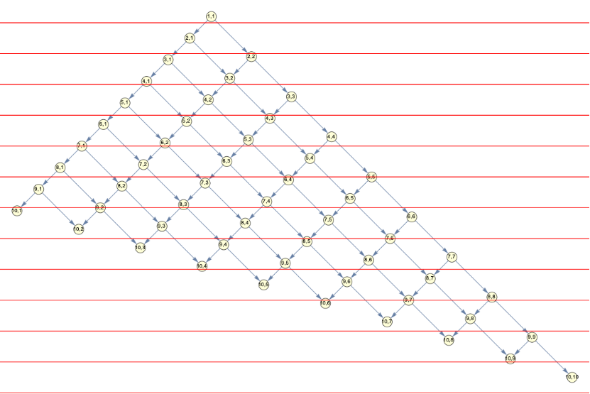
regularCausalGraphPlot[10,1,0.3,lorentz[0.3]]
Out[]=
In[]:=
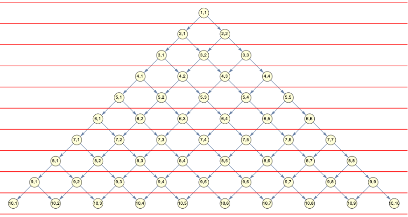
DirectedGraph[Flatten[Table[{v[{i,j}]v[{i+1,j}],v[{i,j}]v[{i+1,j+1}]},{i,10},{j,i}]],VertexCoordinatesCatenate[Table[v[{i,j}]({2(#2-#1/2),-#1}&@@{i,j}),{i,11},{j,i}]],VertexLabels{x_Placed[Row[Riffle[First[x],","]],Center]},VertexSize.33,VertexStyleLightYellow,AspectRatioAutomatic,Epilog{Style[Table[Line[{{-20,k-12},{20,k}}],{k,6.5,-8.5,-1}],Red]}]
Out[]=

In[]:=
RotationMatrix[Iθ]
Out[]=
{{Cosh[θ],-Sinh[θ]},{Sinh[θ],Cosh[θ]}}
In[]:=
{t,x}{t-vx/c^2,x-vt}
Out[]=
{t,x}t-,-tv+x
vx
2
c
Normalize with γ
In[]:=
{t,x}{t-βx,-tβ+x}
Out[]=
{t,x}{t-xβ,x-tβ}
In a string substitution system, we could have a foliation based on the string
In a string substitution system, we could have a foliation based on the string
WM analog
WM analog
Minkowski in SS
Minkowski in SS
We can put a Minkowski norm on here....