LayeredGraphPlot[SubstitutionSystemCausalGraph[{"A""AB","BB""BB"},"A",15],VertexLabelsAutomatic]
In[]:=
Out[]=
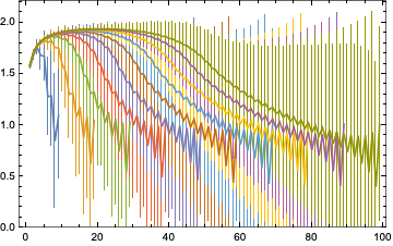
ListLinePlot[Table[LogDifferences@RaggedMeanAround[Values[GraphNeighborhoodVolumes[SubstitutionSystemCausalGraph[{"A""AB","BB""BB"},"A",t]]]],{t,10,100,10}],FrameTrue,PlotRange{0,Automatic}]
In[]:=
Out[]=
ListLinePlot[LogDifferences[{1,2,4,7,12,17,24,31,40,50,61,74,88,104,121,140,160,182,204,228,251,276,300,326,351,377,403,429,455,481,507,533,559,584,608,630,651,670,688,704,719,732,743,753,762,769,775,779,782}]]
In[]:=
Out[]=
RaggedMeanAround[%]
In[]:=
{1,2.78±0.15,5.50±0.22,8.0±0.7,10.5±0.5}
Out[]=
Transpose
Extract[
%[1]
In[]:=
{1,3,6,10,15,21,28,36,44,51,57,62,66,69,71}
Out[]=
Differences[%]
In[]:=
{2,3,4,5,6,7,8,8,7,6,5,4,3,2}
Out[]=
Differences[%]
In[]:=
{1,1,1,1,1,1,0,-1,-1,-1,-1,-1,-1}
Out[]=
GraphNeighborhoodVolumes[SubstitutionSystemCausalGraph[{"A""AB","BB""BB"},"A",30],{1}]
In[]:=
1{1,3,6,10,15,21,28,36,45,55,66,78,91,105,120,136,151,165,178,190,201,211,220,228,235,241,246,250,253,255}
Out[]=
ListLinePlot[LogDifferences[%[1]]]
In[]:=
Out[]=
GraphNeighborhoodVolumes[SubstitutionSystemCausalGraph[{"AA""AAA"},"AA",20],{1}][1]
In[]:=
{1,3,6,11,19,32,51,80,124,189,286,430,643,942,1391,2016,2727,3793,5392,5393}
Out[]=
Ratios[%]//N
In[]:=
{3.,2.,1.83333,1.72727,1.68421,1.59375,1.56863,1.55,1.52419,1.51323,1.5035,1.49535,1.46501,1.47665,1.44932,1.35268,1.39091,1.42157,1.00019}
Out[]=
ListLinePlot[%]
In[]:=
Out[]=
ListLinePlot[LogDifferences[%9]]
In[]:=
Out[]=
GraphNeighborhoodVolumes[SubstitutionSystemCausalGraph[{"A""AA","A""AA","AAA""A"},"AA",20],{1}][1]
In[]:=
{1,3,5,7,11,14,17,23,27,31,39,45,51,63,71,79,95,106,117,139,154,169,199,219,239,279,306,333,387,423,459,531,579,627,723,787,851,979,1065,1151,1323,1438,1553,1783,1937,2091,2399,2605,2811,3223,3498,3773,4323,4690,5057,5791,6281,6771,7751,8405}
Out[]=
ListLinePlot[LogDifferences[%13]]
In[]:=
Out[]=
ParallelMapMonitored[ListLinePlot[LogDifferences[GraphNeighborhoodVolumes[SubstitutionSystemCausalGraph[StringRepeat["A",#1]StringRepeat["A",#2],StringRepeat["A",#1],10],{1}][1]],FrameTrue,PlotLabel{#1,#2}]&@@#&,{{2,3},{2,5},{2,7},{3,4},{3,5},{3,7},{4,5},{4,7},{4,9},{5,6},{5,7},{6,7}}]
In[]:=
$Aborted
Out[]=
ParallelMapMonitored[TimeConstrained[ListLinePlot[LogDifferences[GraphNeighborhoodVolumes[SubstitutionSystemCausalGraph[StringRepeat["A",#1]StringRepeat["A",#2],StringRepeat["A",#1],10],{1}][1]],FrameTrue,PlotLabel{#1,#2}],10]&@@#&,{{2,3},{2,5},{2,7},{3,4},{3,5},{3,7},{4,5},{4,7},{4,9},{5,6},{5,7},{6,7}}]
In[]:=
Out[]=
Map[ListLinePlot[LogDifferences[GraphNeighborhoodVolumes[SubstitutionSystemCausalGraph[StringRepeat["A",#1]StringRepeat["A",#2],StringRepeat["A",#1],20],{1}][1]],FrameTrue,PlotLabel{#1,#2}]&@@#&,{{3,4},{5,7}}]
In[]:=
Out[]=
ParallelMapMonitored[TimeConstrained[ListLinePlot[LogDifferences[GraphNeighborhoodVolumes[SubstitutionSystemCausalGraph[#1,#2,10],{1}][1]],FrameTrue,PlotLabel{#1,#2}],10]&@@#&,{{{"A""BB","BB""AB"},"A"},{{"A""AB","BB""BA"},"A"},{{"AB""AABAB"},"AB"},{{"A""A","A""A","B""BB"},"ABA"},{{"A""A","B""AAAB"},"ABA"},{{"AB""BAABBA"},"AB"},{{"ABA""ABABA"},"ABA"},{{"A""AAB","BAA""A"},"A"},{{"A""BB","BB""ABA"},"A"},{{"A""AA","AAA""AA"},"A"}}]
In[]:=
Out[]=
GraphNeighborhoodVolumes[SubstitutionSystemCausalGraph[{"AA""AAA"},"AA",20],{1}][1]
In[]:=
{1,3,6,11,19,32,51,80,124,189,286,430,643,942,1391,2016,2727,3793,5392,5393}
Out[]=
Ratios[%]//N
In[]:=
{3.,2.,1.83333,1.72727,1.68421,1.59375,1.56863,1.55,1.52419,1.51323,1.5035,1.49535,1.46501,1.47665,1.44932,1.35268,1.39091,1.42157,1.00019}
Out[]=
ListLinePlot[%]
In[]:=
Out[]=
curvedDirectedGraph[n_,neighborhoodSize_,v_:1]:=With[{graph=NeighborhoodGraph[BuckyballGraph[n],v,neighborhoodSize]},With[{center=GraphCenter[graph][[1]]},{HighlightGraph[Graph3D[Select[Reap[BreadthFirstScan[graph,center,{"VisitedVertex"(Sow[#1#2]&)}]][[2,1]],#[[1]]≠#[[2]]&],DirectedEdgesTrue],center],center,GraphNeighborhoodVolumes[graph,{center}][[1]]}]]
In[]:=
ttt=Table[curvedDirectedGraph[Round[7α],Round[25Sqrt[α]]],{α,0.1,2,.1}];
In[]:=
Length[ttt]
In[]:=
20
Out[]=
LayeredGraphPlot[First[#]]&/@ttt
In[]:=
Out[]=
LayeredGraphPlot[]
In[]:=
Out[]=
ttt[[All,3]]
In[]:=
Out[]=
ListLinePlot[LogDifferences/@%76]
In[]:=
Out[]=
ttt[[10,3]]
In[]:=
{1,4,10,19,31,46,64,85,109,136,166,197,231,266,304,342,383,424,468,512,558,604,652,700,748,796}
Out[]=
ListLinePlot[LogDifferences[{1,4,10,19,31,46,64,85,109,136,166,197,231,266,304,342,383,424,468,512,558,604,652,700,748,796}],PlotRange{0,Automatic},FrameTrue]
In[]:=
Out[]=

WM cases

12 steps
ParallelMapMonitored[TimeConstrained[ListLinePlot[LogDifferences[GraphNeighborhoodVolumes[WolframModel[#1,{{0,0},{0,0}},12,"CausalGraph"],{1}][1]],FrameTrue],10]&,{{{x,y},{x,z}}{{y,z},{y,w},{z,w},{w,x}},{{x,y},{y,z}}{{x,y},{y,x},{w,x},{w,z}},{{x,y},{y,z}}{{w,y},{y,z},{z,w},{x,w}}}]
In[]:=
Out[]=
400 steps
ParallelMapMonitored[TimeConstrained[ListLinePlot[LogDifferences[GraphNeighborhoodVolumes[WolframModel[#1,{{0,0,0},{0,0,0}},400,"CausalGraph"],{1}][1]],FrameTrue],10]&,{{{x,y,y},{z,x,u}}{{y,v,y},{y,z,v},{u,v,v}},{{x,y,z},{x,u,v}}{{z,z,w},{w,w,v},{u,v,w}},{{1,1,2},{1,3,4}}{{4,4,3},{2,5,3},{2,5,3}},{{1,1,2},{1,3,4}}{{4,4,5},{5,4,2},{3,2,5}},{{1,2,2},{1,3,4}}{{4,5,5},{5,3,2},{1,2,5}},{{x,y,z},{u,y,v}}{{w,z,x},{z,w,u},{x,y,w}},​​{{1,2,2},{3,2,4}}{{5,3,5},{5,4,4},{4,5,1}},{{1,2,2},{3,1,4}}{{2,3,2},{3,4,4},{2,4,5}},​​{{x,x,y},{z,u,x}}{{u,u,z},{v,u,v},{v,y,x}},{{1,2,1},{1,3,4}}{{4,5,4},{5,4,3},{1,2,5}},{{x,y,z},{x,u,v}}{{x,w,u},{v,w,y},{w,y,z}}}]
In[]:=
Out[]=
ParallelMapMonitored[TimeConstrained[ListLinePlot[LogDifferences[GraphNeighborhoodVolumes[WolframModel[#1,{{0,0,0},{0,0,0}},1500,"CausalGraph"],{1}][1]],FrameTrue],10]&,{{{x,y,y},{z,x,u}}{{y,v,y},{y,z,v},{u,v,v}},{{x,y,z},{x,u,v}}{{z,z,w},{w,w,v},{u,v,w}},{{1,1,2},{1,3,4}}{{4,4,3},{2,5,3},{2,5,3}},{{1,1,2},{1,3,4}}{{4,4,5},{5,4,2},{3,2,5}},{{1,2,2},{1,3,4}}{{4,5,5},{5,3,2},{1,2,5}},{{x,y,z},{u,y,v}}{{w,z,x},{z,w,u},{x,y,w}},​​{{1,2,2},{3,2,4}}{{5,3,5},{5,4,4},{4,5,1}},{{1,2,2},{3,1,4}}{{2,3,2},{3,4,4},{2,4,5}},​​{{x,x,y},{z,u,x}}{{u,u,z},{v,u,v},{v,y,x}},{{1,2,1},{1,3,4}}{{4,5,4},{5,4,3},{1,2,5}},{{x,y,z},{x,u,v}}{{x,w,u},{v,w,y},{w,y,z}}}]
In[]:=
Out[]=
​
WolframModel[{{1,2,1},{1,3,4}}{{4,5,4},{5,4,3},{1,2,5}},{{0,0,0},{0,0,0}},1500,"CausalGraph"]
In[]:=
Out[]=
With[{obj=WolframModel[{{1,2,1},{1,3,4}}{{4,5,4},{5,4,3},{1,2,5}},{{0,0,0},{0,0,0}},1500]},GraphFunctionPlot[obj["CausalGraph"],Association@Thread[Range[obj["EventsCount"]]obj["EventGenerations"]],ColorFunction(ColorData["RedBlueTones"][1-#]&)]]
In[]:=
Out[]=
WolframModel[{{1,2,1},{1,3,4}}{{4,5,4},{5,4,3},{1,2,5}},{{0,0,0},{0,0,0}},300,"LayeredCausalGraph"]
In[]:=
Out[]=
​
cgx=WolframModel[{{1,2,1},{1,3,4}}{{4,5,4},{5,4,3},{1,2,5}},{{0,0,0},{0,0,0}},1500,"CausalGraph"]
In[]:=
Out[]=
HighlightGraph[cgx,NeighborhoodGraph[cgx,1000,10]]
In[]:=
Out[]=
HighlightGraph[cgx,NeighborhoodGraph[cgx,200,10]]
In[]:=
Out[]=
GraphNeighborhoodVolumes[WolframModel[{{1,2,1},{1,3,4}}{{4,5,4},{5,4,3},{1,2,5}},{{0,0,0},{0,0,0}},1500,"CausalGraph"],{1}][1]
In[]:=
{1,3,7,16,33,64,99,132,162,189,217,245,274,302,333,367,404,444,488,536,586,641,702,767,828,891,963,1034,1121,1192,1265,1343,1407,1470,1500}
Out[]=
Ratios[%]//N
In[]:=
{3.,2.33333,2.28571,2.0625,1.93939,1.54688,1.33333,1.22727,1.16667,1.14815,1.12903,1.11837,1.10219,1.10265,1.1021,1.10082,1.09901,1.0991,1.09836,1.09328,1.09386,1.09516,1.09259,1.07953,1.07609,1.08081,1.07373,1.08414,1.06334,1.06124,1.06166,1.04765,1.04478,1.02041}
Out[]=
Differences[%3]
In[]:=
{2,4,9,17,31,35,33,30,27,28,28,29,28,31,34,37,40,44,48,50,55,61,65,61,63,72,71,87,71,73,78,64,63,30}
Out[]=
Differences[%]
In[]:=
{2,5,8,14,4,-2,-3,-3,1,0,1,-1,3,3,3,3,4,4,2,5,6,4,-4,2,9,-1,16,-16,2,5,-14,-1,-33}
Out[]=
ListLinePlot[LogDifferences[%3]]
In[]:=
Out[]=
GraphNeighborhoodVolumes[WolframModel[{{1,2,1},{1,3,4}}{{4,5,4},{5,4,3},{1,2,5}},{{0,0,0},{0,0,0}},5000,"CausalGraph"],{1}][1]
In[]:=
{1,3,7,16,33,68,107,144,180,216,254,294,334,376,419,468,520,578,644,715,794,877,973,1079,1185,1305,1431,1571,1737,1897,2083,2267,2468,2686,2894,3120,3328,3570,3810,4035,4261,4453,4647,4807,4937,5000}
Out[]=
ListLinePlot[LogDifferences[%]]
In[]:=
Out[]=
GraphNeighborhoodVolumes[WolframModel[{{1,2,1},{1,3,4}}{{4,5,4},{5,4,3},{1,2,5}},{{0,0,0},{0,0,0}},10000,"CausalGraph"],{1}][1]
In[]:=
{1,3,7,16,33,68,107,144,182,220,262,306,351,396,445,499,558,625,701,783,873,972,1087,1216,1345,1488,1648,1825,2039,2245,2477,2729,3004,3318,3618,3936,4280,4672,5105,5515,5926,6391,6883,7430,7929,8362,8847,9316,9773,10000}
Out[]=
ListLinePlot[LogDifferences[%]]
In[]:=
Out[]=
GraphNeighborhoodVolumes[WolframModel[{{1,2,1},{1,3,4}}{{4,5,4},{5,4,3},{1,2,5}},{{0,0,0},{0,0,0}},10000,"CausalGraph"]]
In[]:=
Out[]=
RaggedMeanAround[Values[%]]
In[]:=
Out[]=
ListLinePlot[LogDifferences[%]]
In[]:=
Out[]=

Standard 2,4 rule

wmeo=Import["/Users/sw/Dropbox/Physics/Data/22-42-evolution-24.wxf"];
In[]:=
cg24=wmeo["CausalGraph"];
In[]:=
VertexCount[cg24]
In[]:=
3377610
Out[]=
GraphNeighborhoodVolumes[cg24,{1}][1]
In[]:=
{1,3,7,16,35,76,164,349,760,1637,3535,7635,16485,35667,77112,166783,360690,777209,1583477,2591496,3197643,3359399,3377095,3377610}
Out[]=
Ratios[%]//N
In[]:=
{3.,2.33333,2.28571,2.1875,2.17143,2.15789,2.12805,2.17765,2.15395,2.15944,2.15983,2.15914,2.1636,2.162,2.16287,2.16263,2.15478,2.03739,1.63659,1.2339,1.05059,1.00527,1.00015}
Out[]=
ListLinePlot[%]
In[]:=
Out[]=
ListLinePlot[LogDifferences[%126]]
In[]:=
Out[]=
RaggedMeanAround[Values[GraphNeighborhoodVolumes[cg24]]]
In[]:=
GraphNeighborhoodVolumes
In[]:=
Out[]=