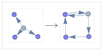
RulePlot[WolframModel[{{0,1},{0,2},{0,3}}{{1,2},{2,3},{3,4},{4,1},{4,3}}]]
In[]:=
Out[]=
GraphPlot[Rule@@@WolframModel[{{0,1},{0,2},{0,3}}{{1,2},{2,3},{3,4},{4,1},{4,3}},Table[0,3,2],20,"FinalState"]]
In[]:=
Out[]=
GraphPlot[Rule@@@#]&/@WolframModel[{{0,1},{0,2},{0,3}}{{1,2},{2,3},{3,4},{4,1},{4,3}},Table[0,3,2],20,"StatesList"]
In[]:=
Out[]=
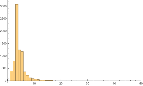
rr30=Graph[Rule@@@WolframModel[{{0,1},{0,2},{0,3}}{{1,2},{2,3},{3,4},{4,1},{4,3}},Table[0,3,2],30,"FinalState"]]
In[]:=
Out[]=
Histogram[VertexDegree[rr30]]
In[]:=
Out[]=
Max[VertexDegree[rr30]]
In[]:=
48
Out[]=
Histogram[VertexDegree[rr30],PlotRangeAll]
In[]:=
Out[]=
GraphPlot[%357]
In[]:=
Out[]=
WolframModel[{{0,1},{0,2},{0,3}}{{1,2},{2,3},{3,4},{4,1},{4,3}},Table[0,3,2],20,"CausalGraph"]
In[]:=
Out[]=
eo25=WolframModel[{{0,1},{0,2},{0,3}}{{1,2},{2,3},{3,4},{4,1},{4,3}},Table[0,3,2],25]
In[]:=
Out[]=
ListLogLogPlotMean
[◼]
HypergraphNeighborhoodVolumes
[eo25["FinalState"],All,Automatic],

In[]:=
Out[]=
NMean
[◼]
HypergraphNeighborhoodVolumes
[eo25["FinalState"],All,Automatic]
In[]:=
{1.,4.3558,15.885,50.6046,141.494,336.478,669.96,1101.18,1508.05,1791.39}
Out[]=
FindFormula[%]
In[]:=
Out[]=
%[r]
In[]:=
Out[]=
FindFit[{1.`,4.3557978196233895`,15.885034687809712`,50.60455896927651`,141.49355797819624`,336.4777006937562`,669.9603567888998`,1101.175421209118`,1508.0455896927651`,1791.388503468781`},ar^d,{a,d},r]
In[]:=
{a2.03447,d2.97131}
Out[]=
Table[FindFit[Take[{1.`,4.3557978196233895`,15.885034687809712`,50.60455896927651`,141.49355797819624`,336.4777006937562`,669.9603567888998`,1101.175421209118`,1508.0455896927651`,1791.388503468781`},n],ar^d,{a,d},r],{n,10}]
In[]:=
FindFit
:Encountered a gradient that is effectively zero. The result returned may not be a minimum; it may be a maximum or a saddle point.
{{a1.,d1.},{a1.,d2.12294},{a0.524266,d3.10341},{a0.225165,d3.90456},{a0.104583,d4.47847},{a0.0756968,d4.68713},{a0.0952019,d4.55343},{a0.210786,d4.12205},{a0.650879,d3.54007},{a2.03447,d2.97131}}
Out[]=
ListLinePlot[{1.`,4.3557978196233895`,15.885034687809712`,50.60455896927651`,141.49355797819624`,336.4777006937562`,669.9603567888998`,1101.175421209118`,1508.0455896927651`,1791.388503468781`}^(1/3)]
In[]:=
Out[]=
eo35=WolframModel[{{0,1},{0,2},{0,3}}{{1,2},{2,3},{3,4},{4,1},{4,3}},Table[0,3,2],35]
In[]:=
Out[]=
Length/@eo35["StatesList"]
In[]:=
{3,5,7,9,13,17,23,31,39,49,67,87,115,157,201,257,343,457,607,805,1053,1369,1799,2345,3089,4037,5271,6897,9009,11767,15461,20161,26355,34409,44967,58695}
Out[]=
FindLinearRecurrence[%]
In[]:=
FindLinearRecurrence[{3,5,7,9,13,17,23,31,39,49,67,87,115,157,201,257,343,457,607,805,1053,1369,1799,2345,3089,4037,5271,6897,9009,11767,15461,20161,26355,34409,44967,58695}]
Out[]=
FindFormula[%371,t]
In[]:=
Out[]=
ListLogPlot[%371,JoinedTrue]
In[]:=
Out[]=
Ratios[%371]//N
In[]:=
{1.66667,1.4,1.28571,1.44444,1.30769,1.35294,1.34783,1.25806,1.25641,1.36735,1.29851,1.32184,1.36522,1.28025,1.27861,1.33463,1.33236,1.32823,1.32619,1.30807,1.30009,1.3141,1.3035,1.31727,1.3069,1.30567,1.30848,1.30622,1.30614,1.31393,1.30399,1.30723,1.3056,1.30684,1.30529}
Out[]=
ListLinePlot[%]
In[]:=
Out[]=
MatrixPlot
[◼]
HypergraphAdjacencyMatrix
[eo35["FinalState"]]
In[]:=
Out[]=
GraphPlot3D[Graph[Rule@@@eo25["FinalState"]]]
In[]:=
Out[]=
fs35=eo35["FinalState"];
In[]:=
NMean
[◼]
HypergraphNeighborhoodVolumes
[fs35,RandomInteger[29000,5],10]
In[]:=
[◼]
GraphNeighborhoodVolumes
Graph
Vertex count: 29347
Edge count: 49226
,{1,2,3},10
In[]:=
Out[]=
eo35["CausalGraph"]
In[]:=
Out[]=
GraphPlot[%]
In[]:=
LayeredGraphPlot[%%]
In[]:=

Vertex Degree Growth

maxVertexDegree[set_]:=Max[Counts[Catenate[Union/@set]]]
In[]:=
​​states=eo35["StatesList"];
In[]:=
​​maxDegrees=maxVertexDegree/@states;
In[]:=
​​ListPlot[maxDegrees]
In[]:=
Out[]=
​
WolframModel[{{0,1},{0,2},{0,3}}{{1,2},{2,3},{3,4},{4,1},{4,3}},Table[0,3,2],20,"CausalGraph"]
In[]:=
Out[]=
GraphPlot3D[%]
In[]:=
LayeredGraphPlot[%%]
In[]:=
Out[]=
Show[%,AspectRatio1]
In[]:=
Out[]=

Random Evolution

randoms=WolframModelEvolutionObject
Generations count: 124
Events count: 10000
Data not in notebook; Store now »
,WolframModelEvolutionObject
Generations count: 117
Events count: 10000
Data not in notebook; Store now »
,WolframModelEvolutionObject
Generations count: 127
Events count: 10000
Data not in notebook; Store now »
,WolframModelEvolutionObject
Generations count: 131
Events count: 10000
Data not in notebook; Store now »
,WolframModelEvolutionObject
Generations count: 107
Events count: 10000
Data not in notebook; Store now »
;
In[]:=

Difference Patterns

WolframModelDifferenceEvolution[{{0,1},{0,2},{0,3}}{{1,2},{2,3},{3,4},{4,1},{4,3}},Table[0,3,2],10,14]
In[]:=
Out[]=
WolframModelDifferenceEvolution[{{0,1},{0,2},{0,3}}{{1,2},{2,3},{3,4},{4,1},{4,3}},Table[0,3,2],17,21]
In[]:=
Out[]=
WolframModelDifferenceEvolution[{{0,1},{0,2},{0,3}}{{1,2},{2,3},{3,4},{4,1},{4,3}},Table[0,3,2],17,24]
In[]:=
Out[]=
WolframModel[{{0,1},{0,2},{0,3}}{{1,2},{2,3},{3,4},{4,1},{4,3}},Table[0,3,2],10]
In[]:=
Out[]=
WolframModelCausalConeSlices[%]
In[]:=
Out[]=
WolframModelCausalConeVolumes[%135]
In[]:=
{{5,31},{9,39},{14,49},{27,67}}
Out[]=
Divide@@@%//N
In[]:=
{0.16129,0.230769,0.285714,0.402985}
Out[]=
WolframModel[{{0,1},{0,2},{0,3}}{{1,2},{2,3},{3,4},{4,1},{4,3}},Table[0,3,2],20]
In[]:=
Out[]=
WolframModelCausalConeSlices[%]
In[]:=
Out[]=
WolframModelCausalConeVolumes[%128,-8]
In[]:=
{{6,157},{16,201},{20,257},{30,343},{63,457},{104,607},{167,805},{264,1053}}
Out[]=
Divide@@@%//N
In[]:=
{0.0382166,0.079602,0.077821,0.0874636,0.137856,0.171334,0.207453,0.250712}
Out[]=
ListLinePlot[%]
In[]:=
Out[]=
(( Like two intersecting light cones ))
Causal-cone-informed graph layout ??

Dimension Computation

WolframModel[{{0,1},{0,2},{0,3}}{{1,2},{2,3},{3,4},{4,1},{4,3}},Table[0,3,2],25];
In[]:=
MeanAround/@TransposeValues
[◼]
HypergraphNeighborhoodVolumes
[%162["FinalState"],All,Automatic]
In[]:=
{1,4.36±0.05,15.89±0.27,50.6±0.9,141.5±2.5,336.±5.,670.±8.,1101.±10.,1508.±9.,1791.±6.}
Out[]=
ListLogLogPlot[%]
In[]:=
Out[]=
vols
In[]:=
1,
1143
263
,
3821
263
,
10509
263
,
24398
263
,
47903
263
,
77513
263
,
104587
263
,
122989
263

Out[]=
ListLinePlot[Table[(Log[vols[[r+1]]]-Log[vols[[r]]])/(Log[r+1]-Log[r]),{r,Length[vols]-1}]]
In[]:=
Out[]=
FindFit[vols,ar^d,{d,a},r]
In[]:=
{d2.97131,a2.03447}
Out[]=