The data structure for g is a list of the form {{x,y,z},{a,b,c}} for each node. Here {x,y,z} are the coordinates of the node, and {a,b,c} are the nodes that have edges coming from this one. The network is drawn on the surface of a sphere of radius 1.
TrivalentFractal[g_,n_]:=With{numpoints=100}, Ifn==0, Graphics3DAbsolutePointSize[1.2],AbsoluteThickness[.25],MapIndexedFunction{y,z},Point[y〚1〛],Functionx,Ifx>First[z],Withgap=&[y〚1〛-g〚x,1〛],TableLine&/@{iy〚1〛+(1-i)g〚x,1〛,(i-gap)y〚1〛+(1-i+gap)g〚x,1〛},{i,gap,1,gap},{}/@y2,g,AspectRatio->Automatic,Boxed->False,ViewPoint->{-1,0,0} ,TrivalentFractal Flatten MapIndexed MapIndexedFunction{x,y},+gx,1, Functionz, Ifz==First[y], 3(x-1)+Position[g〚x,2〛,First[#2]]1,1, 3*(First[#2]-1)+z /@{1,2,3} ,#12& ,g ,1 ,n-1
1
Ceiling[numpoints
#.#
]#
#.#
#
#.#
2
3
1
3
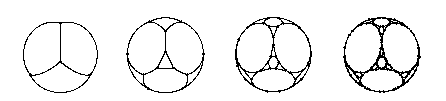
This is the initial state of the fractal network.
TrivalentFractalInitialState={N[{0,0,1}],{2,3,4}},N,0,,{1,3,4},N-,,,{1,2,4},N-,-,,{1,2,3};
3
2
-1
2
3
4
3
4
-1
2
3
4
3
4
-1
2
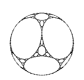
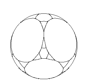
This code displays a specified state of the network.
Show[TrivalentFractal[TrivalentFractalInitialState,4],AspectRatio->Automatic,Boxed->False,ViewPoint->{-1,0,0}];
Show[TrivalentFractal[TrivalentFractalInitialState,2],AspectRatio->Automatic,Boxed->False,ViewPoint->{-1,0,0}];
Table[TrivalentFractal[TrivalentFractalInitialState,i],{i,0,3}];
Show[GraphicsRow[%]];