How Few Basis Functions Does One Need to Approximate Any Wavefunction?
How Few Basis Functions Does One Need to Approximate Any Wavefunction?
Introduction
Introduction
Quantum mechanics tells us that wavefunctions live in an abstract infinite-dimensional space called a Hilbert space. Just as you could describe any 3D vector using 3 perpendicular unit axes, you can describe any wavefunction using a set of orthonormal basis functions.
But here’s a take: what if you don’t use the entire basis? What if you try to approximate a wavefunction using as few basis functions as possible? In this notebook, we'll work with just that: given an arbitrary wavefunction, how few basis functions do we need to represent it accurately?
In this, we will understand how to build orthonormal bases from different function families, how to expand an arbitrary wavefunction such bases, finding the optimal minimal basis set for a given function, how different basis families (like infinite square well eigenfunctions, polynomials, fourier series, etc.) compare in efficiency. Along the way, we'll connect to the essentials, such as probability, energy spectra, and other such concepts. Consider this a rather casual dive into the computational side of quantum representation: part theory, part numerics, and lots of problem solving.
*A/N: Before we get into this, I would like to mention that is supposed to be E subscript n, for some reason capital E doesn't want to work, so we will have to make do with what we've got.*
But here’s a take: what if you don’t use the entire basis? What if you try to approximate a wavefunction using as few basis functions as possible? In this notebook, we'll work with just that: given an arbitrary wavefunction, how few basis functions do we need to represent it accurately?
In this, we will understand how to build orthonormal bases from different function families, how to expand an arbitrary wavefunction such bases, finding the optimal minimal basis set for a given function, how different basis families (like infinite square well eigenfunctions, polynomials, fourier series, etc.) compare in efficiency. Along the way, we'll connect to the essentials, such as probability, energy spectra, and other such concepts. Consider this a rather casual dive into the computational side of quantum representation: part theory, part numerics, and lots of problem solving.
*A/N: Before we get into this, I would like to mention that
n
Why Basis Functions matter
Why Basis Functions matter
Quantum mechanics describes physical systems using wavefunctions, which are mathematical objects that contain all the information about a quantum state. But where do these wavefunctions live? How can we work with them mathematically? The very answer lies in a special kind of mathematical space called a Hilbert space.
An Introduction to Hilbert Space
An Introduction to Hilbert Space
Imagine you’re working with regular 3D vectors. You have an origin, three perpendicular axes (x, y, z) and any vector can be written as a combination of unit vectors along these axes:
v=vxî + vyĵ + vzk
v=vxî + vyĵ + vzk
vectorPlot=Graphics3D[{{Thick,Red,Arrow[{{0,0,0},{2,0,0}}]},{Thick,Green,Arrow[{{0,0,0},{0,3,0}}]},{Thick,Blue,Arrow[{{0,0,0},{0,0,1}}]},{Black,Thickness[0.01],Arrow[{{0,0,0},{2,3,1}}]},{Dashed,Red,Arrow[{{0,0,0},{2,0,0}}]},{Dashed,Green,Arrow[{{2,0,0},{2,3,0}}]},{Dashed,Blue,Arrow[{{2,3,0},{2,3,1}}]},Text[Style["i",Bold,18],{2.2,0,0}],Text[Style["j",Bold,18],{0,3.2,0}],Text[Style["k",Bold,18],{0,0,1.2}],Text[Style["v = 2i + 3j + 1k",Bold,16],{2.5,3.5,1.5}]},BoxedTrue,AxesTrue,AxesLabel{"x","y","z"},PlotLabelStyle["3D Vector Decomposition: Basis Analogy",Bold,16],ViewPoint{3,-2,1},Lighting"Neutral"]
Out[]=

Hilbert space is the infinite-dimensional generalization of this idea. Instead of three dimensions, we have (typically) infinitely many. Instead of vectors, we have wavefunctions (functions like ψ(x)) that satisfy certain mathematical properties. The key features of Hilbert space are: Inner products: For any two wavefunctions ψ(x) and ϕ(x), we can define: ⟨ψ∣ϕ⟩=∫ψ∗(x)ϕ(x)dx
ClearAll["Global`*"];
x=Subdivide[0,1,399];L=1;
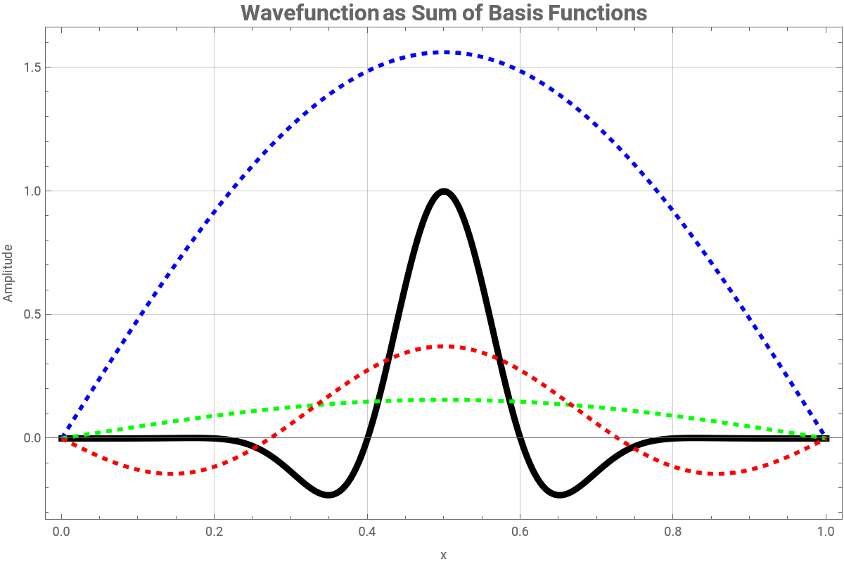
psi=Exp[-50*(x-0.5)^2]*Sin[5*Pi*x];
basis1=Sqrt[2/L]*Sin[Pi*x/L];basis2=Sqrt[2/L]*Sin[2*Pi*x/L];basis3=Sqrt[2/L]*Sin[3*Pi*x/L];
c1=Total[basis1*psi]*(L/399);c2=Total[basis2*psi]*(L/399);c3=Total[basis3*psi]*(L/399);
curve1=psi;curve2=c1*basis1;curve3=c1*basis1+c2*basis2;curve4=c1*basis1+c2*basis2+c3*basis3;
wavefunctionPlot=ListLinePlot[{Transpose[{x,curve1}],Transpose[{x,10*curve2}],Transpose[{x,curve3}],Transpose[{x,curve4}]},PlotStyle{{Black,Thickness[0.008]},{Blue,Thickness[0.005],Dashed},{Green,Thickness[0.005],Dashed},{Red,Thickness[0.005],Dashed}},PlotLegends{"Original ψ(x)","10× c₁φ₁(x) (scaled)","c₁φ₁(x) + c₂φ₂(x)","c₁φ₁(x) + c₂φ₂(x) + c₃φ₃(x)"},FrameTrue,FrameLabel{"x","Amplitude"},PlotLabelStyle["Wavefunction as Sum of Basis Functions",Bold,16],GridLinesAutomatic,ImageSize600,PlotRangeAll]
Out[]=


This measures how much ψ and ϕ overlap.Norm (Length):∥ψ∥=⟨ψ∣ψ⟩
This gives us a way to measure the “size” of a wavefunction.
Completeness: Every sensible wavefunction can be represented in this space, and limits of sequences of wavefunctions stay within the space.
Completeness: Every sensible wavefunction can be represented in this space, and limits of sequences of wavefunctions stay within the space.
Hermitian Operators: The basis Generators
Hermitian Operators: The basis Generators
In quantum mechanics, measurable quantities (observables) like position, momentum and energy are represented by Hermitian operators. These operators have two crucial properties:Real eigenvalues: When you measure an observable, you get a real number. Orthogonal eigenfunctions: The eigenfunctions corresponding to different eigenvalues are orthogonal. For example, the Hamiltonian operator H^ (which represents energy) satisfies: (x)=(x)
Ĥ
ϕn
E
nϕn
In[]:=
L=1;x=Subdivide[0,L,399];energies={1,4,9,16};eigenfunctions=Table[Sqrt[2/L]*Sin[n*Pi*x/L],{n,1,4}];
plot1=ListLinePlot[Table[Transpose[{x,eigenfunctions[[n]]+energies[[n]]}],{n,1,4}],PlotStyle{{Red,Thickness[0.005]},{Blue,Thickness[0.005]},{Green,Thickness[0.005]},{Purple,Thickness[0.005]}},PlotLegends{"φ₁(x), E₁ = 1","φ₂(x), E₂ = 4","φ₃(x), E₃ = 9","φ₄(x), E₄ = 16"},FrameTrue,FrameLabel{"Position (x)","Energy/Amplitude"},PlotLabelStyle["Hamiltonian Eigenfunctions: Ĥφₙ = Eₙφₙ",Bold,16],GridLinesAutomatic,AspectRatio0.6,ImageSize600]
The Complete Basis Set Theorem
The Complete Basis Set Theorem
Think of it like this: just as any 3D vector can be built from î,ĵ,k̂, any wavefunction can be built from a complete set of basis functions.
Why Finite Approximations Work
Why Finite Approximations Work
Intro To Orthonormalization and Orthonormalizing Wavefunctions
Intro To Orthonormalization and Orthonormalizing Wavefunctions
Okay, now that we understand why we need orthonormal basis functions, let’s learn how to make them. There are two main methods: starting from scratch with arbitrary functions, or using the ready-made bases that quantum systems provide.
The Gram Schmidt Process
The Gram Schmidt Process
What if we have a set of functions that seem useful but aren’t orthogonal? The Gram-Schmidt process is what we use to transforms any linearly independent set of functions into an orthonormal set.
The Method
The Method
Let’s say we start with functions f1(x),f2(x),f3(x),… that are linearly independent but not orthogonal. We want to create orthonormal functions ϕ1(x),ϕ2(x),ϕ3(x),... .
To do this, we will follow these simple steps:
To do this, we will follow these simple steps:
Why This Works Geometrically
Why This Works Geometrically
Imagine you’re in 3D space with three non-orthogonal vectors. Gram-Schmidt is like:
“You gotta take the first vector and normalize it, that’s gonna be your first basis vector. Then you take the second vector and subtract any component that points along the first, so now that’s gonna be perpendicular to the first right? Then you just do the same with the third vector, but you subtract the components along both previous vectors, so now its perpendicular to both of the previous vectors!”
The same idea works in function space!!
“You gotta take the first vector and normalize it, that’s gonna be your first basis vector. Then you take the second vector and subtract any component that points along the first, so now that’s gonna be perpendicular to the first right? Then you just do the same with the third vector, but you subtract the components along both previous vectors, so now its perpendicular to both of the previous vectors!”
The same idea works in function space!!
A Quick Example
A Quick Example
Quantum Bases: Starting from Eigenfunctions
Quantum Bases: Starting from Eigenfunctions
Again, sometimes we don’t need to orthogonalize from scratch- quantum mechanics gives us ready-made orthonormal bases for a low cost of $0.00!
The Infinite Square Well Basis
The Infinite Square Well Basis
The Harmonic Oscillator Basis
The Harmonic Oscillator Basis
Why are these special?? How can I choose my basis wisely?
Why are these special?? How can I choose my basis wisely?
Choosing your basis wisely
To be honest, the “best” basis depends on your wavefunction:
If your wavefunction is confined to [0,L] that go to zero at boundaries, then its best to use the infinite square well basis.
If your wavefunction is rather Gaussian-like or is a function on an infinite domain, then you should probably use the harmonic oscillator basis.
A fourier basis is perfect for periodic functions, and a polynomial (Gram-Schmidt) is flexible, but may converge slowly.
To be honest, the “best” basis depends on your wavefunction:
If your wavefunction is confined to [0,L] that go to zero at boundaries, then its best to use the infinite square well basis.
If your wavefunction is rather Gaussian-like or is a function on an infinite domain, then you should probably use the harmonic oscillator basis.
A fourier basis is perfect for periodic functions, and a polynomial (Gram-Schmidt) is flexible, but may converge slowly.
Expanding an Arbitrary Wavefunction in the Orthonormal Basis
Expanding an Arbitrary Wavefunction in the Orthonormal Basis
Now we get to the core of the matter: taking any wavefunction ψ(x) and expressing it in terms of our carefully constructed orthonormal basis. This is where all the good work happens, and where we can finally work on our question about minimal basis sets.
The Expansion Formula
The Expansion Formula
The Truncation Tradeoff: Accuracy vs complexity
The Truncation Tradeoff: Accuracy vs complexity
Parseval’s Identity
Parseval’s Identity
The Coefficient Decay Rate
The Coefficient Decay Rate
Defining Good Enough
Defining Good Enough
Finding the Optimal N
Finding the Optimal N
The Optimization Challenge
The Optimization Challenge
Two Optimization problems
Two Optimization problems
The Algorithm And How We Find The Minimum
The Algorithm And How We Find The Minimum
Here’s a step-by-step on how you can find the optimal basis representation:
Different Bases Gives Different Results
Different Bases Gives Different Results
The Algorithm
The Algorithm
Case Study: Infinite Square Well
Case Study: Infinite Square Well
Ready Made Basis Set
Ready Made Basis Set
Probability Interpretation
Probability Interpretation
Energy Spectrum Connection
Energy Spectrum Connection
Measuring Success with Error Analysis
Measuring Success with Error Analysis
The Error Norm
The Error Norm
Convergence Plots
Convergence Plots
This plot explains how each curve shows how the error decreases as we include more basis functions. The steeper the curve, the more efficient the basis.
The knee represents the optimal balance between accuracy and complexity; the point where adding more terms yields minimal improvement.
Basis Efficiency Comparison:
When we overlay multiple convergence curves, we can directly compare basis families:
When we overlay multiple convergence curves, we can directly compare basis families:
The chart makes it clear: some bases need far fewer terms to reach the same accuracy. For our Gaussian wavepacket, the infinite square well basis converges fastest, while the polynomial lags behind.
The chart makes it clear: some bases need far fewer terms to reach the same accuracy. For our Gaussian wavepacket, the infinite square well basis converges fastest, while the polynomial lags behind.
Understanding the Patterns
Understanding the Patterns
The Big Picture
The Big Picture
Error analysis and convergence plots aren’t simply just mathematical formalities — they’re the connection between abstract theory and practical computation.
When we ask “How few basis functions do we need?”, the convergence plot gives us the answer. It shows us, term by term, how our approximation improves. It tells us when we’ve captured enough of the wavefunction’s norm, and when adding more terms is just overkill. In the context of quantum mechanics, this has real physical meaning. Each term we add corresponds to including another energy eigenstate in our description. The convergence plot shows us which energy levels matter, and how many we need to include to describe the system to within our desired accuracy.
When we ask “How few basis functions do we need?”, the convergence plot gives us the answer. It shows us, term by term, how our approximation improves. It tells us when we’ve captured enough of the wavefunction’s norm, and when adding more terms is just overkill. In the context of quantum mechanics, this has real physical meaning. Each term we add corresponds to including another energy eigenstate in our description. The convergence plot shows us which energy levels matter, and how many we need to include to describe the system to within our desired accuracy.
Compare which basis would win
Compare which basis would win
We’ve now seen how individual bases perform, but the real question is: If you had to pick one basis to rule them all, which one would it be?
TLDR: There is no single winner.
TLDR: There is no single winner.
Fourier Basis Vs Polynomial Basis vs Quantum Well Basis
Fourier Basis Vs Polynomial Basis vs Quantum Well Basis
Results: Why no single basis always wins
Results: Why no single basis always wins
Gaussian Wavepacket (Smooth, localized)):
Error at N=10:
Quantum Well: 0.003
Fourier: 0.003
Polynomial: 0.015
Winner: Quantum Well / Fourier (tie!)
Loser: Polynomial
Observations: The Gaussian is smooth and vanishes at the boundaries; it’s literally designed for the quantum well basis. The Fourier basis also loves smooth, localized functions because they’re band-limited in frequency space. Polynomials struggle because they have to work extra hard to make the approximation vanish at the edges, something the other bases do for free. So while a Gaussian wavepacket is made of many energy eigenstates, they’re concentrated around a specific energy range. The quantum well basis captures this naturally because index n maps directly to energy.
Error at N=10:
Quantum Well: 0.003
Fourier: 0.003
Polynomial: 0.015
Winner: Quantum Well / Fourier (tie!)
Loser: Polynomial
Observations: The Gaussian is smooth and vanishes at the boundaries; it’s literally designed for the quantum well basis. The Fourier basis also loves smooth, localized functions because they’re band-limited in frequency space. Polynomials struggle because they have to work extra hard to make the approximation vanish at the edges, something the other bases do for free. So while a Gaussian wavepacket is made of many energy eigenstates, they’re concentrated around a specific energy range. The quantum well basis captures this naturally because index n maps directly to energy.
----------------------------------------------------------------------------------------------------------------------------------------------------------------------------------------------------------------------------------------------------------------------------------
Square Pulse (Discontinuous)
Error at N=20:
Quantum Well: 0.12
Fourier: 0.14
Polynomial: 0.11
Winner: Polynomial (barely)
Loser: Everyone (it’s painful)
Observations: Discontinuities are a great equalizer; everyone converges slowly. The polynomial basis edges out a win because it doesn’t care about boundary conditions (the square pulse doesn’t vanish at the edges), but all three are struggling. The Fourier basis exhibits the classic Gibbs phenomenon: oscillations near the discontinuity that don’t go away. Another observation to note is that a square pulse contains all frequencies equally. That’s why you need so many terms. No basis can cheat this- its a fundamental property of Fourier analysis. The discontinuity forces 1/n coefficient decay in any basis of smooth functions.
Square Pulse (Discontinuous)
Error at N=20:
Quantum Well: 0.12
Fourier: 0.14
Polynomial: 0.11
Winner: Polynomial (barely)
Loser: Everyone (it’s painful)
Observations: Discontinuities are a great equalizer; everyone converges slowly. The polynomial basis edges out a win because it doesn’t care about boundary conditions (the square pulse doesn’t vanish at the edges), but all three are struggling. The Fourier basis exhibits the classic Gibbs phenomenon: oscillations near the discontinuity that don’t go away. Another observation to note is that a square pulse contains all frequencies equally. That’s why you need so many terms. No basis can cheat this- its a fundamental property of Fourier analysis. The discontinuity forces 1/n coefficient decay in any basis of smooth functions.
----------------------------------------------------------------------------------------------------------------------------------------------------------------------------------------------------------------------------------------------------------------------------------
Highly Oscillatory Gaussian:
Error at N=15:
Quantum Well: 0.008
Fourier: 0.008
Polynomial: 0.045
Winner: Quantum Well / Fourier
Loser: Polynomial (by a mile)
Observations: The wavefunction wiggles rapidly- its all about high frequencies. Both the quantum well and Fourier bases have built-in high-frequency modes (just use larger n). In the case of polynomials, they need to combine many low-frequency modes to approximate a high-frequency wiggle. Its like building an SEM with parts from the junkyard: possible (somehow), but inefficient. Now, oscillation frequency ≈ basis index n. For a wavefunction that oscillates 20 times, you need n ≈ 20 terms in the right basis. Polynomials don’t have a clean frequency-index relationship, so they need many more terms to achieve the same accuracy.
Highly Oscillatory Gaussian:
Error at N=15:
Quantum Well: 0.008
Fourier: 0.008
Polynomial: 0.045
Winner: Quantum Well / Fourier
Loser: Polynomial (by a mile)
Observations: The wavefunction wiggles rapidly- its all about high frequencies. Both the quantum well and Fourier bases have built-in high-frequency modes (just use larger n). In the case of polynomials, they need to combine many low-frequency modes to approximate a high-frequency wiggle. Its like building an SEM with parts from the junkyard: possible (somehow), but inefficient. Now, oscillation frequency ≈ basis index n. For a wavefunction that oscillates 20 times, you need n ≈ 20 terms in the right basis. Polynomials don’t have a clean frequency-index relationship, so they need many more terms to achieve the same accuracy.
----------------------------------------------------------------------------------------------------------------------------------------------------------------------------------------------------------------------------------------------------------------------------------
Triangle Wave (Continuous, not smooth)
Error at N=15:
Quantum Well: 0.018
Fourier: 0.018
Polynomial: 0.032
Winner: Quantum Well / Fourier
Runner-up: Polynomial
Observations: The triangle wave is continuous, but has a kink (derivative discontinuity). Its coefficients decay as 1/n^2, giving error ~1/N. The sinusoidal bases exploit this cleanly. Polynomials do okay but need more terms to capture the sharp corner. The kink means high frequencies are still present, but they’re weaker than in a discontinuity. The better the basis matches the function’s smoothness class, the faster the convergence. The sinusoidal bases have the right “built-in” decay rate for this function class.
Triangle Wave (Continuous, not smooth)
Error at N=15:
Quantum Well: 0.018
Fourier: 0.018
Polynomial: 0.032
Winner: Quantum Well / Fourier
Runner-up: Polynomial
Observations: The triangle wave is continuous, but has a kink (derivative discontinuity). Its coefficients decay as 1/n^2, giving error ~1/N. The sinusoidal bases exploit this cleanly. Polynomials do okay but need more terms to capture the sharp corner. The kink means high frequencies are still present, but they’re weaker than in a discontinuity. The better the basis matches the function’s smoothness class, the faster the convergence. The sinusoidal bases have the right “built-in” decay rate for this function class.
Why No Single Basis Always Wins
Why No Single Basis Always Wins
Let’s visualize this with a heatmap of “terms needed for 95% accuracy”. This heatmap would show a checkerboard pattern; no single basis is best for all wavefunctions:
Physical Interpretation Matters:
Sometimes the “best” basis isn’t the one that converges fastest, but the one that makes the physics clear.
----------------------------------------------------------------------------------------------------------------------------------------------------------------------------------------------------------------------------------------------------------------------------------
Quantum well basis: Coefficients = probability amplitudes for energy measurements
Fourier basis: Coefficients = probability amplitudes for momentum measurements
Polynomial basis: Coefficients = ??? (mathematically convenient, but what do they mean?)
If you care about energy, use the energy basis. If you care about momentum, use the momentum basis. If you just want a good approximation and don’t care about interpretation, pick whichever converges fastest for your specific wavefunction.
Sometimes the “best” basis isn’t the one that converges fastest, but the one that makes the physics clear.
----------------------------------------------------------------------------------------------------------------------------------------------------------------------------------------------------------------------------------------------------------------------------------
Quantum well basis: Coefficients = probability amplitudes for energy measurements
Fourier basis: Coefficients = probability amplitudes for momentum measurements
Polynomial basis: Coefficients = ??? (mathematically convenient, but what do they mean?)
If you care about energy, use the energy basis. If you care about momentum, use the momentum basis. If you just want a good approximation and don’t care about interpretation, pick whichever converges fastest for your specific wavefunction.
Match the Tool to the Task
Match the Tool to the Task
A Practical Guide
A Practical Guide
When you’re faced with a new wavefunction:
First, look at the boundaries. Does ψ(0)=ψ(L)=0? If yes, quantum well basis is a strong contender.
Second, assess smoothness. Is it analytic? Smooth? Continuous? Discontinuous? Smoother is better in any basis.
Third, consider oscillations. If it wiggles a lot, you need high frequencies. Make sure your basis has them.
Fourth, think about physics. Do you want energy probabilities? Use the energy basis. Momentum? Use Fourier.
Finally, when in doubt, test. Compute the first few coefficients in different bases. See which ones decay fastest. A quick numerical experiment beats hours of theoretical hand-wringing.
First, look at the boundaries. Does ψ(0)=ψ(L)=0? If yes, quantum well basis is a strong contender.
Second, assess smoothness. Is it analytic? Smooth? Continuous? Discontinuous? Smoother is better in any basis.
Third, consider oscillations. If it wiggles a lot, you need high frequencies. Make sure your basis has them.
Fourth, think about physics. Do you want energy probabilities? Use the energy basis. Momentum? Use Fourier.
Finally, when in doubt, test. Compute the first few coefficients in different bases. See which ones decay fastest. A quick numerical experiment beats hours of theoretical hand-wringing.
Conclusion
Conclusion