Optimal Contour Path Finder for Complex Integrals
Optimal Contour Path Finder for Complex Integrals
Introduction
Introduction
Navigating complex integrals needs accuracy, and finding the right paths is essential. Using methods like the residue theorem, adjusting contours, and handling branch cuts helps us find simpler ways to solve these integrals. Picking the right contour not only makes the process easier but also leads to better solutions for complex integrals.
Theory and Approach
Theory and Approach
A Basic Introduction to Contour Integration
A Basic Introduction to Contour Integration
To evaluate complex integrals, we use contour integration. Complex contour integration is a method used to solve integrals by moving along a specific path in the complex plane. The path you choose, called a contour, is important because it helps navigate around points where the function may behave strangely, like singularities or branch cuts. These points can cause problems, so picking the right contour ensures calculations work smoothly.
Residue Theorem
Residue Theorem
One of the most useful tools in contour integration is the Residue Theorem. It lets you evaluate complex integrals by adding up the residues of singularities inside the contour. This approach makes calculations much easier, especially when dealing with multiple poles. To make the process efficient, it’s important to choose a contour that captures the key residues while avoiding difficult singularities or branch points.
Consider the function f(z) = 1 / ((z - 1) * (z + 2)). This function has poles at z = 1 and z = -2 (You will be seeing this function a lot). To apply residue theorem, we need to
compute the residues at these poles and evaluate the integral along a contour that encloses both poles.
compute the residues at these poles and evaluate the integral along a contour that encloses both poles.
In[]:=
f[z_]:=1/((z-1)(z+2))
To find the residues at the poles z = 1 and z = -2, we use the Residue function. The residues are given by:
In[]:=
residue1=Residue[f[z],{z,1}]residue2=Residue[f[z],{z,-2}]
Out[]=
1
3
Out[]=
-
1
3
Using residue theorem, the integral of f (z) around a contour enclosing both poles can be computed as (2\pi i\) times the sum of the residues . Here' s how we can compute this integral :
In[]:=
contour=Circle[{0,0},3];
In[]:=
totalResidue=residue1+residue2
Out[]=
0
In[]:=
integralValue=2PiI*totalResidue
Out[]=
0
In[]:=
integralValue
Out[]=
0
Residue theorem is a powerful method for evaluating complex integrals by focusing on residues. For instance, consider a different function g(z) = e^z / ((z - 2) * (z - 3i)). This function has poles at z = 2 and z = 3i. We can apply the Residue Theorem in a similar manner:
In[]:=
g[z_]:=Exp[z]/((z-2)(z-3I))
In[]:=
residueAt2=Residue[g[z],{z,2}];residueAt3i=Residue[g[z],{z,3I}];
In[]:=
totalResidueNew=residueAt2+residueAt3i;
In[]:=
integralValueNew=2PiI*totalResidueNew;
In[]:=
{residueAt2,residueAt3i,integralValueNew}
Out[]=
+,--,2--++π
2
13
3
13
2
2
13
3
13
3
2
13
3
13
3
2
13
3
13
2
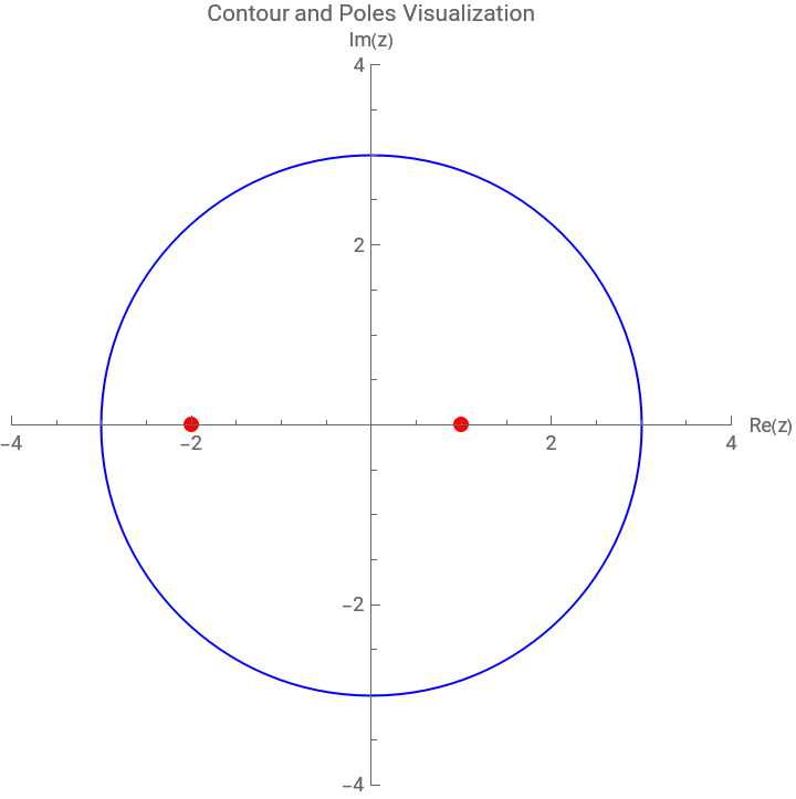
Visualizing the function and its singularities can enhance understanding . For the function f (z) = 1 / ((z - 1) * (z + 2)), we can plot the contour and highlight the poles . This helps in understanding how the contour encloses the singularities .
In[]:=
polesPlot=Graphics[{Red,PointSize[Large],Point[{1,0}],Point[{-2,0}],Blue,Circle[{0,0},3]}];
In[]:=
Show[polesPlot,PlotRange->{{-4,4},{-4,4}},PlotLabel->"Contour and Poles Visualization",Axes->True,AxesOrigin->{0,0},Ticks->Automatic,AxesLabel->{"Re(z)","Im(z)"}]
Out[]=
In[]:=
Singularities and Branch Cuts
Singularities and Branch Cuts
Singularities, such as poles, and branch cuts are points or lines in the complex plane where the function behaves non-analytically. Identifying these features is crucial for determining the optimal contour. A path that passes through or near these points must be chosen carefully to either exploit the residues (in the case of poles) or avoid crossing branch cuts, which would complicate the integral.
In[]:=
f[z_]:=1/((z-1)Sqrt[z+2])
In[]:=
branchCut={{-2,0},{-5,0}};
In[]:=
singularity={1,0};
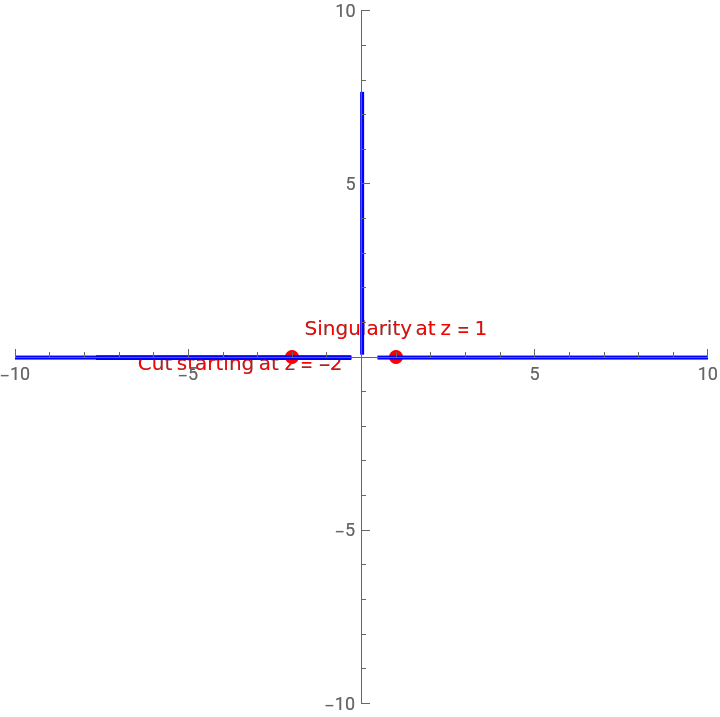
The following visualization shows the function f(z) = 1 / ((z - 1) * √(z + 2)), which helps us understand how the function behaves in the complex plane. This function has a branch cut that goes from z = -2 to negative infinity, with a singularity at z = 1.
In[]:=
ParametricPlot[{Re[f[x]],Im[f[x]]},{x,-4,2},PlotLegends->Automatic,PlotRange->{{-10,10},{-10,10}},AspectRatio->1,PlotStyle->{Thick,Blue},Prolog->{Red,PointSize[Large],Point[singularity],Point[{branchCut[[1]]}],Text["Singularity at z = 1",{1,0.5},{0,-1}],Text["Cut starting at z = -2",{-3.5,-0.5},{0,-1}]}]
Out[]=
Modus Operandi: How We can Optimize Contour Path Finding
Modus Operandi: How We can Optimize Contour Path Finding
The approach to finding the optimal contour involves several steps :
1. Identify Singularities: First, we locate all the singularities and branch points in the complex plane.
2. Evaluate Potential Contours: We then consider various potential contours that could enclose these singularities, each with its own set of pros and cons.
3. Compute Residues: For each potential contour, we’ll calculate the residues of the enclosed singularities.
4. Optimize the Path: Select the contour that maximizes the sum of these residues while minimizing the path length and avoiding unnecessary complications from branch cuts .
1. Identify Singularities: First, we locate all the singularities and branch points in the complex plane.
2. Evaluate Potential Contours: We then consider various potential contours that could enclose these singularities, each with its own set of pros and cons.
3. Compute Residues: For each potential contour, we’ll calculate the residues of the enclosed singularities.
4. Optimize the Path: Select the contour that maximizes the sum of these residues while minimizing the path length and avoiding unnecessary complications from branch cuts .
Implementation
Implementation
Introduction
Introduction
Finding the best contour for evaluating complex integrals can make calculations easier and more accurate. In this section, we introduce the OptimalContourPathFinder, a tool that helps identify the best path by looking at different possible contours and optimizing them based on the contributions from residues.
Defining the Function and Its Singularities
Defining the Function and Its Singularities
To begin, we once again define the complex function:f (z) = 1 / ((z - 1) * (z + 2)) . This function has poles at z = 1andz = -2.
In[]:=
f[z_]:=1/((z-1)(z+2))singularities={1,-2}
Out[]=
{1,-2}
Here, f[z_] is the complex function we will integrate, and singularities represents the locations of the poles of the function. These singularities are important as they determine the contours we need to consider.
If you Can’t Find it, Make it: Creating the Optimal Pathfinder
If you Can’t Find it, Make it: Creating the Optimal Pathfinder
Next, we create the Optimal Contour Path Finder. This evaluates different contours, computes the integral along each contour, and selects the one that provides the most efficient path for integration. The process involves computing residues at the singularities, evaluating integrals along candidate contours, and identifying the optimal contour based on the integral values .
In[]:=
f[z_]:=1/((z-1)(z+2))singularities={1,-2};
Function code
Function code
BRANCH CUTS FUNCTION:
BRANCH CUTS FUNCTION:
SPLIT CONTOUR FUNCTION:
SPLIT CONTOUR FUNCTION:
OPTIMAL CONTOUR PATH FINDER :
OPTIMAL CONTOUR PATH FINDER :
Examples and Visualizations
Examples and Visualizations
Here are a couple examples that use the OptimalContourPathFinder function:
1- Simple Circular Contours Around Singularities:
1- Simple Circular Contours Around Singularities:
We’ll consider a function with poles (singularities) and test circular contours around them. The function being 1/(z - 1) (z + 1), where the singularities are at z = 1 and z = -1 and our circular contours being centered at z = 0 with radius 2, z = 0 with radius 1.5 and z = 0 with radius 1.
Define the function f(z) :
Define the singularities:
Define the three circular contours
Run the OptimalContourPathFinder on the function:
The function automatically displays a graph for you!
This will produce a plot of the singularities and the optimal contour path , based on the maximum integral value . Since it’ s a simple contour selection case, it will just show the optimal contour along with the singularities at z = 1 and z = −1.
2- Contours with Winding Numbers Around a Singular Pole
2- Contours with Winding Numbers Around a Singular Pole
In this example, we’ll use the same function f(z) but allow the contours to wind around the singularity multiple times (winding numbers)., where our circle has a radius 2 winding once, twice and three times.
Lets first define the same function and singularities
and define a contour that winds around the singularities
Use winding numbers 1, 2, and 3
(The plot above shows a much more concise visualization as compared to the native function’s plot)
3- Handling Branch Cuts with Split Contours
3- Handling Branch Cuts with Split Contours
First lets define a function with a branch cut along the negative real axis
and define the branch cut
*Assume this function detects branch cuts*
Run the OptimalContourPathFinder
And finally, we display the optimal contour and graph
This will display two possible contours :
One that avoids the branch cut and circles around z = 1, and another that crosses the branch cut, splitting the contour into segments . The function will automatically handle the branch cut and compute the integral correctly.
One that avoids the branch cut and circles around z = 1, and another that crosses the branch cut, splitting the contour into segments . The function will automatically handle the branch cut and compute the integral correctly.
Conclusion
Conclusion
In this study, we explored how the Optimal Contour Path Finder can be applied to complex integrals, particularly by focusing on singularities, branch cuts, and winding numbers.
For future work, it would be amazing to test a variety of contour shapes, such as spirals, astroids, and lemniscates, to see how they perform in different scenarios. This would lead to a more complete and deeper understanding of contour optimization.
For future work, it would be amazing to test a variety of contour shapes, such as spirals, astroids, and lemniscates, to see how they perform in different scenarios. This would lead to a more complete and deeper understanding of contour optimization.
Bibliography
Bibliography
Encyclopedia Britannica, inc. (n.d.). Singularity. Encyclopedia Britannica. https://www.britannica.com/topic/singularity-complex-functions
Rosales, R. R. (1999, October 11). Branch points and branch cuts (18.04, MIT). https://math.mit.edu/classes/18.305/Notes/n00Branch_Points_B_Cuts.pdf
Weisstein, Eric W. “Residue Theorem.” From MathWorld--A Wolfram Web Resource. https://mathworld.wolfram.com/ResidueTheorem.html
Weisstein, Eric W. “Contour Integration.” From MathWorld--A Wolfram Web Resource. https://mathworld.wolfram.com/ContourIntegration.html
Stalker, J. (1998). In Complex Analysis: Fundamentals of the Classical Theory of Functions. (pp. 77–78).
Encyclopedia Britannica, inc. (n.d.). Singularity. Encyclopedia Britannica. https://www.britannica.com/topic/singularity-complex-functions
Rosales, R. R. (1999, October 11). Branch points and branch cuts (18.04, MIT). https://math.mit.edu/classes/18.305/Notes/n00Branch_Points_B_Cuts.pdf
Weisstein, Eric W. “Residue Theorem.” From MathWorld--A Wolfram Web Resource. https://mathworld.wolfram.com/ResidueTheorem.html
Weisstein, Eric W. “Contour Integration.” From MathWorld--A Wolfram Web Resource. https://mathworld.wolfram.com/ContourIntegration.html
Stalker, J. (1998). In Complex Analysis: Fundamentals of the Classical Theory of Functions. (pp. 77–78).