Second order point statistics are homogeneity measures of how uniformly the points are distributed within the observation window. They are used to study data locations in relation to other data points.

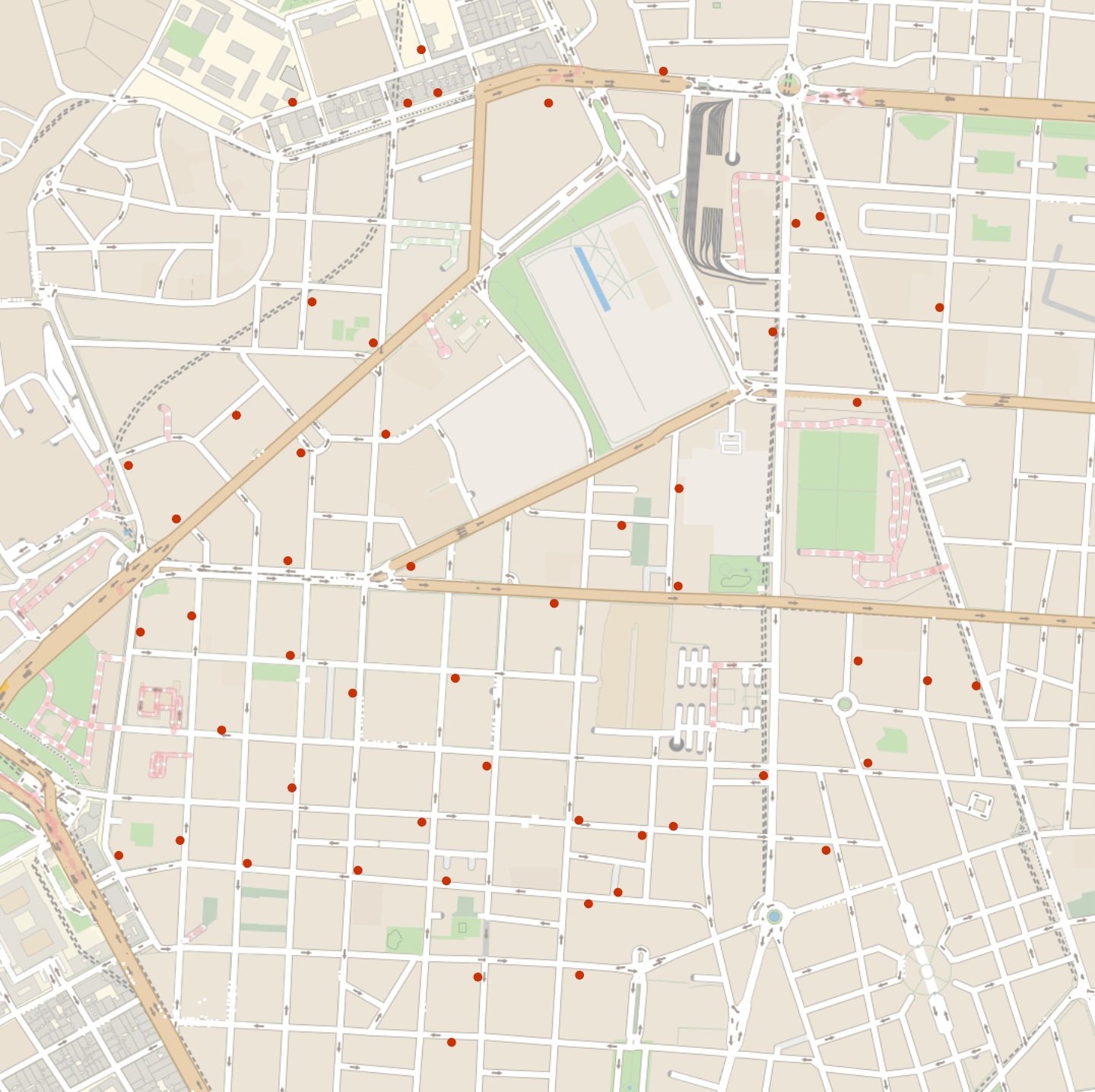
Location of pharmacies in a part of Madrid city:

In[1]:=

Create SpatialPointData with the observation region inferred from the data points:

In[2]:=

Out[2]=

Visualize the data:

In[3]:=

Out[3]=

Test if the locations are random:

In[4]:=

Out[4]=

In[5]:=

Out[5]=

So it looks like the locations are random, but are they arbitrarily close to each other? For the answer we compute NearestNeighborG:

In[6]:=

Out[6]=

Compute maximum radius for the point statistics function:

In[7]:=

Out[7]=

Maximum radius magnitude in meters:

In[8]:=

Out[8]=

Visualize:

In[9]:=

Out[9]=

So the plot of the NearestNeighborG of the data indicates that pharmacies cannot be arbitrarily close to each other. The limiting distance is called hardcore radius and such data can be modelled by a HardcorePointProcess:

In[10]:=

Out[10]=

Estimated hardcore radius is:

In[11]:=

Out[11]=

Since the pharmacies cannot be arbitrarily close to each other we can ask what is the expected number of pharmacies within given distance from a given pharmacy - that is how big is the competition within the given radius. This can be answered using another point statistics function - RipleyK:

In[12]:=

Out[12]=

The product of the value of RipleyK at r and the mean point density gives the expected number of points within distance r of a typical point, not counting the point itself:

In[13]:=

Out[13]=

What is the radius within which the expected number of pharmacies is at least 1?

In[14]:=

Out[14]=

The expected number of pharmacies is at least 1 within the radius of at least 149 meters.

Now let’s compute the probability of encountering a pharmacy within given distance starting from a random location in the observation region which is not a point of the data. The point statistics to do so is EmptySpaceF:

In[15]:=

Out[15]=

Value of EmptySpaceF at r gives exactly the probability of finding a point within distance r of an arbitrary location which is typically not a point of data set:

In[16]:=

Out[16]=

The probability of encountering a pharmacy within 100 meters of a random location in the observation region is:

In[17]:=

Out[17]=