Wolfram Cloud
Resource Object
Example Resource
Affine Nonlinear Systems
Source Notebook
Affine Nonlinear Systems
Examples
Example Notebook
Open in Cloud
Download Notebook
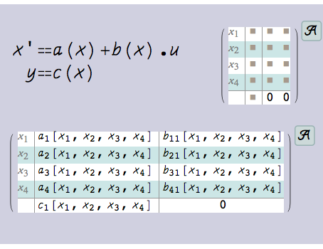
Affine systems are nonlinear systems that are linear in the input. They can be specified in multiple ways and can also be converted to other systems models.
A system specified using an ODE:
I
n
[
1
]
:
=
A
f
f
i
n
e
S
t
a
t
e
S
p
a
c
e
M
o
d
e
l
[
m
x
'
'
[
t
]
+
c
[
x
]
x
'
[
t
]
+
k
[
x
]
F
[
t
]
,
x
[
t
]
,
F
[
t
]
,
x
[
t
]
,
t
]
O
u
t
[
1
]
=
x
.
1
[
t
]
x
.
2
[
t
]
0
x
.
2
[
t
]
-
k
[
x
]
-
c
[
x
]
x
.
2
[
t
]
m
1
m
x
.
1
[
t
]
0
A system specified using its components:
I
n
[
2
]
:
=
A
f
f
i
n
e
S
t
a
t
e
S
p
a
c
e
M
o
d
e
l
[
{
{
f
1
[
x
1
,
x
2
]
,
f
2
[
x
1
,
x
2
]
}
,
{
{
g
1
1
[
x
1
,
x
2
]
}
,
{
g
2
1
[
x
1
,
x
2
]
}
}
,
{
h
1
[
x
1
,
x
2
]
}
}
,
{
x
1
,
x
2
}
]
O
u
t
[
2
]
=
x
1
f
1
[
x
1
,
x
2
]
g
1
1
[
x
1
,
x
2
]
x
2
f
2
[
x
1
,
x
2
]
g
2
1
[
x
1
,
x
2
]
h
1
[
x
1
,
x
2
]
0
Systems obtained from other systems models:
I
n
[
3
]
:
=
A
f
f
i
n
e
S
t
a
t
e
S
p
a
c
e
M
o
d
e
l
/
@
a
1
1
a
1
2
b
1
1
a
2
1
a
2
2
b
2
1
c
1
1
c
1
2
0
,
1
-
2
s
+
2
s
,
x
1
f
1
[
x
1
,
x
2
]
+
u
1
g
1
1
[
x
1
,
x
2
]
x
2
f
2
[
x
1
,
x
2
]
+
u
1
g
2
1
[
x
1
,
x
2
]
h
1
[
x
1
,
x
2
]
O
u
t
[
3
]
=
x
1
a
1
1
x
1
+
a
1
2
x
2
b
1
1
x
2
a
2
1
x
1
+
a
2
2
x
2
b
2
1
c
1
1
x
1
+
c
1
2
x
2
0
,
x
.
1
x
.
2
0
x
.
2
2
x
.
2
1
x
.
1
0
,
x
1
f
1
[
x
1
,
x
2
]
g
1
1
[
x
1
,
x
2
]
x
2
f
2
[
x
1
,
x
2
]
g
2
1
[
x
1
,
x
2
]
h
1
[
x
1
,
x
2
]
0
A
N
o
n
l
i
n
e
a
r
S
t
a
t
e
S
p
a
c
e
M
o
d
e
l
that is not input linear is approximated:
I
n
[
4
]
:
=
A
f
f
i
n
e
S
t
a
t
e
S
p
a
c
e
M
o
d
e
l
x
1
f
1
[
x
1
,
x
2
,
u
1
]
x
2
f
2
[
x
1
,
x
2
,
u
1
]
h
1
[
x
1
,
x
2
,
u
1
]
O
u
t
[
4
]
=
x
1
f
1
[
x
1
,
x
2
,
0
]
(
0
,
0
,
1
)
f
1
[
x
1
,
x
2
,
0
]
x
2
f
2
[
x
1
,
x
2
,
0
]
(
0
,
0
,
1
)
f
2
[
x
1
,
x
2
,
0
]
h
1
[
x
1
,
x
2
,
0
]
(
0
,
0
,
1
)
h
1
[
x
1
,
x
2
,
0
]
A linear
A
f
f
i
n
e
S
t
a
t
e
S
p
a
c
e
M
o
d
e
l
is exactly converted to linear systems models:
I
n
[
5
]
:
=
a
s
s
m
=
x
1
x
1
+
x
2
1
x
2
x
1
1
x
1
0
;
I
n
[
6
]
:
=
{
S
t
a
t
e
S
p
a
c
e
M
o
d
e
l
[
a
s
s
m
]
,
T
r
a
n
s
f
e
r
F
u
n
c
t
i
o
n
M
o
d
e
l
[
a
s
s
m
]
}
O
u
t
[
6
]
=
1
1
1
1
0
1
1
0
0
,
1
+
s
.
-
1
-
s
.
+
2
s
.
In general, affine models are approximated during conversion to linear systems models:
I
n
[
7
]
:
=
a
s
s
m
=
x
1
x
1
+
x
2
+
x
1
x
2
1
x
2
x
1
1
+
x
2
x
1
0
;
I
n
[
8
]
:
=
{
S
t
a
t
e
S
p
a
c
e
M
o
d
e
l
[
a
s
s
m
]
,
T
r
a
n
s
f
e
r
F
u
n
c
t
i
o
n
M
o
d
e
l
[
a
s
s
m
]
}
O
u
t
[
8
]
=
1
1
1
1
0
1
1
0
0
,
1
+
s
.
-
1
-
s
.
+
2
s
.
The conversion to a
N
o
n
l
i
n
e
a
r
S
t
a
t
e
S
p
a
c
e
M
o
d
e
l
is exact:
I
n
[
9
]
:
=
N
o
n
l
i
n
e
a
r
S
t
a
t
e
S
p
a
c
e
M
o
d
e
l
x
1
f
1
[
x
1
,
x
2
]
g
1
1
[
x
1
,
x
2
]
x
2
f
2
[
x
1
,
x
2
]
g
2
1
[
x
1
,
x
2
]
h
1
[
x
1
,
x
2
]
0
O
u
t
[
9
]
=
x
1
f
1
[
x
1
,
x
2
]
+
u
1
g
1
1
[
x
1
,
x
2
]
x
2
f
2
[
x
1
,
x
2
]
+
u
1
g
2
1
[
x
1
,
x
2
]
h
1
[
x
1
,
x
2
]
"
"
Source Metadata
Publisher Information
Contributed By:
Wolfram Staff