Created on 9/14/25 by Nick Abboud
A short mathematica tutorial
A short mathematica tutorial
Mathematica is useful for symbolic computation. That means, roughly, that it can solve equations in terms of variables without having to plug in numbers first. To see how it works, we will use it to solve question 2 from the discussion worksheet.
Mathematica is useful for symbolic computation. That means, roughly, that it can solve equations in terms of variables without having to plug in numbers first. To see how it works, we will use it to solve question 2 from the discussion worksheet.
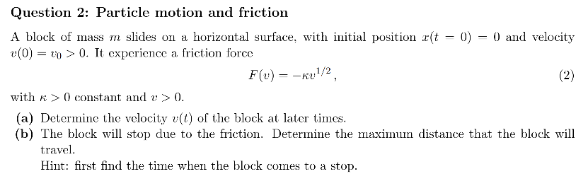
Part (a)
Part (a)
From Newton’s second law, we have the differential equationmdvdt=-κ1/2v.To solve this, we will rely on the built-in Mathematica function DSolve. This is our first lesson: for typical use, Mathematica is just a collection of built-in functions that can be used to perform common tasks.To get started, click below where indicated. Your cursor will look like this when you’re hovering over the right spot: .vvv click here
From Newton’s second law, we have the differential equation.To solve this, we will rely on the built-in Mathematica function DSolve. This is our first lesson: for typical use, Mathematica is just a collection of built-in functions that can be used to perform common tasks.To get started, click below where indicated. Your cursor will look like this when you’re hovering over the right spot: .vvv click here
m=-κ
dv
dt
1/2
v
^^^ click here
After clicking there, you can start typing to create a new cell. Type DSolve[ (case sensitive, no closing bracket), and then press the down arrow key. This opens up a cheat sheet for DSolve[]. Notice that the way you provide arguments to the function can differ based on your intended usage, as is typical in Mathematica. At the top of the list, there is a little icon of an open book. This button opens up the documentation for DSolve[]. Mathematica has great documentation with plenty of examples.
Now let’s actually use DSolve[] to solve the problem. In the cell below, type DSolve[{m v’[t] == -k Sqrt[v[t]], v[0]==v0},v[t],t] and press Shift+Enter to run the cell.
(*putcodebelow*)
Note that a space between variables and/or functions denotes multiplication, like in m v'[t] . If you wrote mv'[t], then Mathematica would think you meant the derivative of a function called mv . Also make sure you use == here, which is used to test equality, instead of =, which declares equality.
Let’s pick this apart a bit more. The first argument we gave to DSolve[] is {m v’[t] == -k Sqrt[v[t]], v[0] == v0}, which is a list of two equations. The first equation is the differential equation itself. We used the built-in function Sqrt[], but we could have written v[t]^(1/2) instead. The second equation is the initial condition, which DSolve[] that the velocity at time 0 is a variable called v0. The second argument, namely v[t], specifies the differential equation’s dependent variable, and the third argument t is the independent variable.
Now let’s look at the output. When you pressed Shift+Enter, you should have gotten the following output:
Out[]=
v[t]-4kmtv0,v[t]+4kmtv0
2
k
2
t
v0
+42
m
4
2
m
2
k
2
t
v0
+42
m
4
2
m
Mathematica has found two solutions. That is very strange--we only expected one! Let’s try to figure this out. First, let’s have Mathematica simplify this output so it’s easier to look at. Copy-and-paste the entire output and put it between the square brackets below, and then press Shift+Enter to run the cell.
Mathematica has found two solutions. That is very strange--we only expected one! Let’s try to figure this out. First, let’s have Mathematica simplify this output so it’s easier to look at. Copy-and-paste the entire output and put it between the square brackets below, and then press Shift+Enter to run the cell.
Simplify[]
If copying and pasting seems like bad form, you can store the output of DSolve[] in a variable called sol like so. Try evaluating the cell below.
If copying and pasting seems like bad form, you can store the output of DSolve[] in a variable called sol like so. Try evaluating the cell below.
In[]:=
sol=DSolve[{mv'[t]==-kSqrt[v[t]],v[0]==v0},v[t],t];Simplify[sol]
To try to understand why we got two solutions, and which one is correct, let’s plot them. To do so, we have to provide numerical values for m, k, and v0. In the cell below, type sol/.{m->1, k->2, v0->3} and execute it.
To try to understand why we got two solutions, and which one is correct, let’s plot them. To do so, we have to provide numerical values for m, k, and v0. In the cell below, type sol/.{m->1, k->2, v0->3} and execute it.
(*putcodebelow*)
What you have just done is called applying a rule. More precisely, {m -> 1, k -> 2, v0 -> 3} is a list of three rules meaning “replace m by 1, k by 2, and v0 by 3”. The notation /. means “apply the rule on the right to the thing on the left”. This construction is used all the time.Now let’s plot both of the solutions on the same plot. Do to this, usePlot[{v1, v2}, {t, 0, 3}, AxesLabel->{“t”,“v[t]”}, PlotLegends->{“solution 1”,“solution 2”}]You’ll have to replace the placeholders v1 and v2 by the outputs of the previous command, i.e. by 14(12-83t+42t) and 14(12+83t+42t), respectively. You can do this by copy-and-pasting or with an appropriate rule replacement.
What you have just done is called applying a rule. More precisely, {m -> 1, k -> 2, v0 -> 3} is a list of three rules meaning “replace m by 1, k by 2, and v0 by 3”. The notation /. means “apply the rule on the right to the thing on the left”. This construction is used all the time.Now let’s plot both of the solutions on the same plot. Do to this, usePlot[{v1, v2}, {t, 0, 3}, AxesLabel->{“t”,“v[t]”}, PlotLegends->{“solution 1”,“solution 2”}]You’ll have to replace the placeholders v1 and v2 by the outputs of the previous command, i.e. by (12-8) and (12+8), respectively. You can do this by copy-and-pasting or with an appropriate rule replacement.
1
4
3
t+42
t
1
4
3
t+42
t
(*putcodebelow*)
Note that the argument {t, 0, 3} tells Mathematica to plot for values of t between 0 and 3. The option AxesLabel specifies the labels for the axes. The option PlotLegends specifies a legend for the plot, so we can tell which curve is which. There are many more stylistic options for plots.From this plot, we see that in solution 2 the velocity increases after t=0, which is clearly unphysical, because the minus sign in the force law -k Sqrt[v[t]] should make v[t] decrease over time. Mathematica got overzealous trying to provide the most general solution and seems to have interpreted Sqrt[v[t]] to mean ±Sqrt[v[t]]. In fact, you can verify by hand that solution 2 isn’t actually a solution of the differential equation. This happens from time to time, so it’s very important to check that the answers provided by Mathematica make sense.We also see that, in solution 1, after v[t] reaches zero, it starts to climb up again! That can’t be right, and it also stems from Mathematica’s over-interpretation of Sqrt. However, you can verify that solution 1 is indeed a solution to Newton’s 2nd law until it reaches v[t]=0. That is, up until v[t] reaches zero, it is given byv[t]=2k t-2 m v04 2m.
Note that the argument {t, 0, 3} tells Mathematica to plot for values of t between 0 and 3. The option AxesLabel specifies the labels for the axes. The option PlotLegends specifies a legend for the plot, so we can tell which curve is which. There are many more stylistic options for plots.From this plot, we see that in solution 2 the velocity increases after t=0, which is clearly unphysical, because the minus sign in the force law -k Sqrt[v[t]] should make v[t] decrease over time. Mathematica got overzealous trying to provide the most general solution and seems to have interpreted Sqrt[v[t]] to mean ±Sqrt[v[t]]. In fact, you can verify by hand that solution 2 isn’t actually a solution of the differential equation. This happens from time to time, so it’s very important to check that the answers provided by Mathematica make sense.We also see that, in solution 1, after v[t] reaches zero, it starts to climb up again! That can’t be right, and it also stems from Mathematica’s over-interpretation of Sqrt. However, you can verify that solution 1 is indeed a solution to Newton’s 2nd law until it reaches v[t]=0. That is, up until v[t] reaches zero, it is given byv[t]=.
2
k t-2 m
v0
4
2
m
Part (b)
Part (b)
To find the time when the block stops moving, we want to solve the equation 2k t-2 m v04 2m==0 for t. Try to do this using the built-in function Solve[]. Hint: look at the documentation for Solve[], as described earlier.
To find the time when the block stops moving, we want to solve the equation ==0 for t. Try to do this using the built-in function Solve[]. Hint: look at the documentation for Solve[], as described earlier.
2
k t-2 m
v0
4
2
m
(*putcodebelow*)
You should find that the stopping time is 2 m v0k. (If you got two solutions and both of them are the same, that’s just because Mathematica wanted to tell you that the root has multiplicity 2.)Now to find the maximum distance, we first need to solve the differential equationx'[t]==2k t-2 m v04 2mwith the initial condition x[0]==0. Do this with DSolve[], using part (a) as a guide.
You should find that the stopping time is . (If you got two solutions and both of them are the same, that’s just because Mathematica wanted to tell you that the root has multiplicity 2.)Now to find the maximum distance, we first need to solve the differential equationwith the initial condition x[0]==0. Do this with DSolve[], using part (a) as a guide.
2 m
v0
k
x'[t]==
2
k t-2 m
v0
4
2
m
(*putcodebelow*)
You should find that x[t] is given by t 2k 2t-6 k m t v0+12 2m v012 2m. Now, referring back to part (a) if needed, apply the rule t->2 m v0k to this expression to find the maximum distance traveled by the block. You might need to Simplify[] the result.
You should find that x[t] is given by . Now, referring back to part (a) if needed, apply the rule t-> to this expression to find the maximum distance traveled by the block. You might need to Simplify[] the result.
t -6 k m t v0
2
k
2
t
v0
+12 2
m
12
2
m
2 m
v0
k
(*putcodebelow*)
Prologue
Prologue
We have only touched on the very basics here. Mathematica can do just about any mathematical operation you can think of. However, as we saw in this tutorial, it’s very important to check the output critically, because Mathematica can sometimes behave unexpectedly. Plotting things is a great way to check results, and Mathematica has all kinds of different plotting functions.
If you choose to use Mathematica or other symbolic computation software on the homework, please keep in mind that you must provide a clear copy of the code you used to generate the answer to receive full credit.
I think the best way to learn more about Mathematica is to try to use it. If you know roughly what you want it to do (e.g. perform an integral), then you can always find pertinent info in the Mathematica documentation or on Stack Exchange. Generations of people have been frustrated by Mathematica before, so you can greatly minimize your suffering by googling!