Out[]=
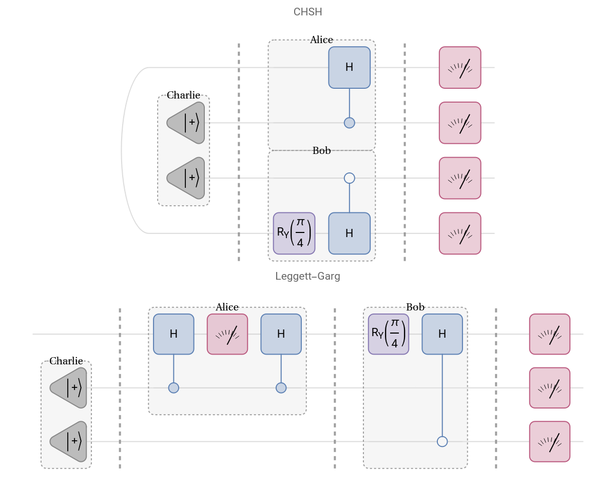
Leggett-Garg (LG) inequality is a temporal version of the much more famous Clauser-Horne-Shimony-Holt (CHSH) inequality, which has already been explored quite in-depth here.
This short post is about how spatial and temporal entanglements differ and what they have in common.
This short post is about how spatial and temporal entanglements differ and what they have in common.
As already can be seen from the hero image with different kinds of separation between Alice and Bob, the CHSH setup exploits vertical entanglement with participants performing their part of the experiment separated by (potentially enormous) spatial distance in parallel. The LG setup, on the other hand, features entanglement in the horizontal direction, with the main parties separated in time and firing their devices sequentially, one after another.
The CHSH circuit involves sharing an entangled Bell pair between Alice and Bob, which results in additional correlation between measurement outcomes due to celebrated non-local quantum effects and violates the CHSH inequality or wins the CHSH game more often than possible purely by classical means.
Analogously, one can construct the LG circuit serving the same purpose of a game and with the same game rules as its counterpart. It even has the same components, with the sole exception of Alice performing an extra operation of undoing her measurement basis preparation to restore their common communication line with Bob to its original orientation.
The CHSH circuit involves sharing an entangled Bell pair between Alice and Bob, which results in additional correlation between measurement outcomes due to celebrated non-local quantum effects and violates the CHSH inequality or wins the CHSH game more often than possible purely by classical means.
Analogously, one can construct the LG circuit serving the same purpose of a game and with the same game rules as its counterpart. It even has the same components, with the sole exception of Alice performing an extra operation of undoing her measurement basis preparation to restore their common communication line with Bob to its original orientation.
Install the freshest version of the Wolfram Quantum Framework first:
In[]:=
PacletInstall["https://www.wolfr.am/DevWQCF",ForceVersionInstall->True]<<Wolfram`QuantumFramework`
Out[]=
PacletObject

Instead of analyzing the all-in-one circuit, it would be beneficial to decompose all its explicit conditionals into four separate cases. All those controlled gates effectively choose one of two bases in which Alice and Bob perform their measurement. On a Bloch sphere, they form two perpendicular sets rotated by 45 degrees:
Out[]=


Let’s construct these bases first:
In[]:=
(*Alicebases*)x1=QuantumBasis[];x2=QuantumBasis["X"];(*Bobbases*)y1=QuantumOperator["RY"[Pi/4]]@x1;y2=QuantumOperator["RY"[-Pi/4]]@x1;
Now we can use these to make custom measurement operators with some natural choice of eigenvalues for this problem (1 and -1):
In[]:=
QuantumMeasurementOperator[y1->{1,-1}]
Out[]=
QuantumMeasurementOperator

For example, measuring default empty register state with the first of Alice’s bases, we get the corresponding measurement with a single target qubit:
|0〉
In[]:=
QuantumMeasurementOperator[x1->{1,-1}][]
Out[]=
QuantumMeasurement

If we then apply Bob’s first measurement to it, the target now contains the same qubit twice with the total of four possible outcomes with different probabilities:
In[]:=
m=N@QuantumMeasurementOperator[y1->{1,-1}]@QuantumMeasurementOperator[x1->{1,-1}][]
Out[]=
QuantumMeasurement

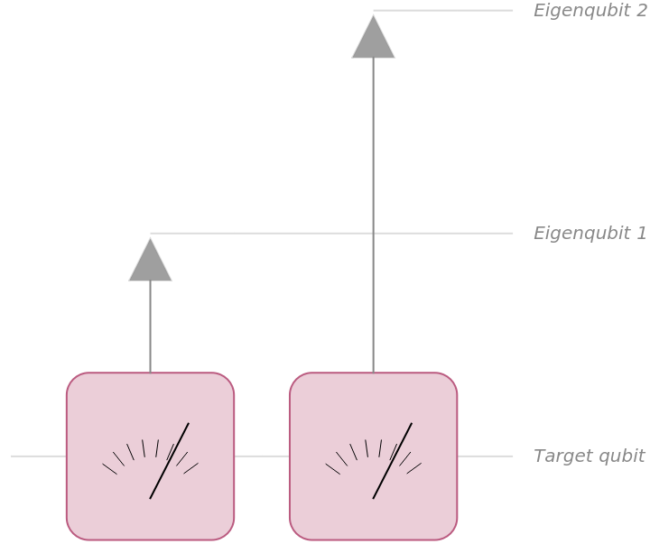
A careful observer would notice that something weird is happening, as probability for Alice getting -1 should always be 0. There is a slight technical problem here, and probabilities are indeed incorrect. Measurement probabilities, by default, are always shown in the current basis of the target qubit, but after sequentially measuring the same qubit with two different bases, we need probabilities in those corresponding bases, not both in the same last one! The quick workaround for this is to instead show probabilities for the corresponding eigenqubits by setting a special label to the measurement:
In[]:=
QuantumMeasurement[m,"Label"->"Eigen"]
Out[]=
QuantumMeasurement

Out[]=
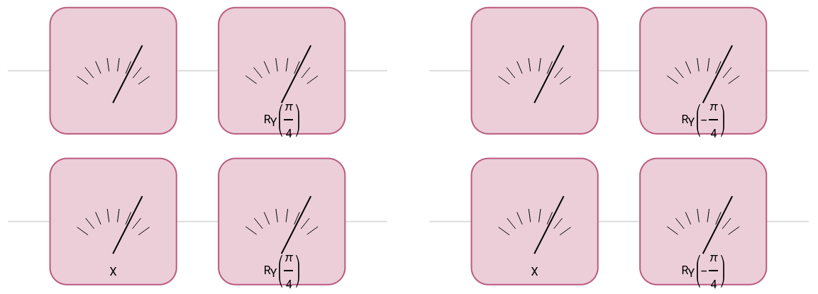
We can now compute probabilities and construct categorical distributions for all four different choices of bases:
In[]:=
distributions=Table[QuantumMeasurement[N@QuantumMeasurementOperator[{y1,y2}[[y]]->{1,-1}]@QuantumMeasurementOperator[{x1,x2}[[x]]->{1,-1}][],"Label"->"Eigen"]["MultivariateDistribution"],{x,2},{y,2}]
Out[]=
CategoricalDistribution,CategoricalDistribution,CategoricalDistribution,CategoricalDistribution
Which correspond to the following circuits consisting of just two measurements each:
Out[]=
Now we can also easily compute correlations between Alice and Bob’s measurement outcomes for all of these cases:
In[]:=
correlations=Table[Sum[abPDF[distributions[[x,y]],{a,b}],{a,{1,-1}},{b,{1,-1}}],{x,2},{y,2}]
Out[]=
{{0.707107,0.707107},{0.707107,-0.707107}}
The LG inequality, as well as the CHSH inequality, both have the exact same form, including a term that maximally combines these correlations, which requires a change of sign for the last one:
In[]:=
Tablecorrelations[[x,y]],{x,2},{y,2}
(x-1)(y-1)
(-1)
Out[]=
{{0.707107,0.707107},{0.707107,0.707107}}
And summing them up:
Out[]=

In[]:=
TotalTablecorrelations[[x,y]],{x,2},{y,2},All
(x-1)(y-1)
(-1)
Out[]=
2.82843
The inequality then taking the following form:
Out[]=

And the above result of have successfully violated it.
2
2
≈2.82843While having the same form, CHSH and LG inequalities have different assumptions. CHSH requires realism and locality, while LQ similarly requires realism, but instead of locality, it requires non-invasive measurements and sometimes also something called an induction (https://arxiv.org/pdf/1304.5133.pdf). Therefore, as a result of violating both inequalities, any realist would conclude that quantum computation is non-local and with measurements undeniably affecting its target system.
We can also similarly compute the LG term using a single circuit with the help of Charlie, the referee, who is responsible for choosing one of the four setups and corresponding correlations above:
And computing probability of winning in the LG game is as expected ~85%, which is higher than classical limit of 75%:
CITE THIS NOTEBOOK
CITE THIS NOTEBOOK
Time entanglement and Leggett-Garg inequality
by Nikolay Murzin
Wolfram Community, STAFF PICKS, February 13, 2024
https://community.wolfram.com/groups/-/m/t/3121574
by Nikolay Murzin
Wolfram Community, STAFF PICKS, February 13, 2024
https://community.wolfram.com/groups/-/m/t/3121574