Everyone has heard of qubits - quantum bits, states that can be anything “between” and , maybe someone even heard of qudits - d-dimensional quantum states describing the superposition of basis states . But is there anything in between these integer dimensions, some alternative computational model? It turns out there is a natural extension of quantum theory to any square root of integer dimension, like etc. With qubits, qutrits and qudits in general only occupy perfect square positions in this sequence: . These are called squbits, squtrits, squadrits and so on, with squadrits being the same as the usual qubit.


d

2
,3
,5
4
,9
and16
PacletInstall["https://www.wolfr.am/DevWQCF",ForceVersionInstall->True]<<Wolfram`QuantumFramework`
Why qubit is a squadrit or-dimensional? Recall that any qubit in general has 3 degrees of freedom, you can either think of them as the number of real components of its Hermitian density matrix with unit trace:
4
Out[]//MatrixForm=
a | b+c |
b-c | 1-a |
Out[]//MatrixForm=
0.430292 | -0.419426-0.108298 |
-0.419426+0.108298 | 0.569708 |
Or as 3-dimensional Bloch vector:
Out[]=

However, in one specific sense, it is also advantageous to attribute a 4-dimensional probability distribution to a qubit, which also has 3 degrees of freedom, because probabilities typically need to sum up to 1.
There is no unique way of doing it, but the general tool for this is MIC-POVM or Minimally Information-ally Complete Positive Operator Valued Measurement.
In[]:=
povm=QuantumMeasurementOperator["RandomPOVM"]
Out[]=
QuantumMeasurementOperator


These complete measurement operators fully describe the quantum state by probabilities of measuring it with a set of basis states, which is 4 in the case of qubits:
2
d
In[]:=
ρ=QuantumState["RandomMixed"]measurement=povm[ρ]
Out[]=
QuantumState

Out[]=
QuantumMeasurement

In[]:=
measurement["Probabilities"]
Out[]=
|〉0.100727,|〉0.537653,|〉0.155027,|〉0.206593
ℛ
1
ℛ
2
ℛ
3
ℛ
4
Probabilities fully describing the state means that this representation is equivalent to some change of basis of the original density matrix or of equivalent doubled state representation:
In[]:=
basis=QuditBasis[Inverse[Outer[Tr@*Dot,#,#,1]].#&@povm["POVMElements"]]
Out[]=
QuditBasis

In[]:=
QuantumState[ρ["Double"],basis]["Amplitudes"]
Out[]=
|0〉0.100727,|1〉0.537653,|2〉0.155027,|3〉0.206593
In[]:=
QuantumWeylTransform[QuantumState[ρ["Double"],basis]]==ρ
Out[]=
True
This means that any quantum computation can be carried away in this probabilistic basis without complex numbers. Where any unitary gate, measurement or channel appropriately converted:
In[]:=
U=QuantumOperator["RandomUnitary"];M=QuantumMeasurementOperator[];
In[]:=
QuantumBasis[QuditBasis[2],basis]
Out[]=
QuantumBasis

In[]:=
=Chop@QuantumState[ρ["Double"],basis]["StateVector"];=Chop@QuantumOperator[U["Double"],QuantumBasis[basis,basis]]["Matrix"];ℳ=Chop@QuantumOperator[M["Double"]["DiscardExtraQudits"],QuantumBasis[QuditBasis[2],basis]]["Matrix"];
In[]:=
//MatrixForm
Out[]//MatrixForm=
0.100727 |
0.537653 |
0.155027 |
0.206593 |
In[]:=
//MatrixForm
Out[]//MatrixForm=
0.583119 | 0.132284 | -0.0819103 | 0.097187 |
-1.25087 | 1.21766 | 0.314059 | -0.212161 |
2.84976 | -0.581655 | 0.552362 | 0.242314 |
-1.182 | 0.231706 | 0.215489 | 0.87266 |
In[]:=
ℳ//MatrixForm
Out[]//MatrixForm=
5.61106 | -0.923088 | -0.0428991 | 1.071 |
-4.61106 | 1.92309 | 1.0429 | -0.0710036 |
In[]:=
U[ρ]["Probability"]
Out[]=
|0〉0.507603,|1〉0.492397
In[]:=
ℳ..//Normal
Out[]=
{0.507603,0.492397}
There are some better choices of basis to pick, for qubits the Tetrahedron basis is perhaps the most natural:
In[]:=
basis=QuditBasis["Tetrahedron"];=Chop@QuantumState[ρ["Double"],basis]["StateVector"];=Chop@QuantumOperator[U["Double"],QuantumBasis[basis,basis]]["Matrix"];ℳ=Chop@QuantumOperator[M["Double"]["DiscardExtraQudits"],QuantumBasis[QuditBasis[2],basis]]["Matrix"];
In[]:=
ℳ//MatrixForm
Out[]//MatrixForm=
2 | 0 | 0 | 0 |
-1 | 1 | 1 | 1 |
In[]:=
ℳ..//Normal
Out[]=
{0.507603,0.492397}
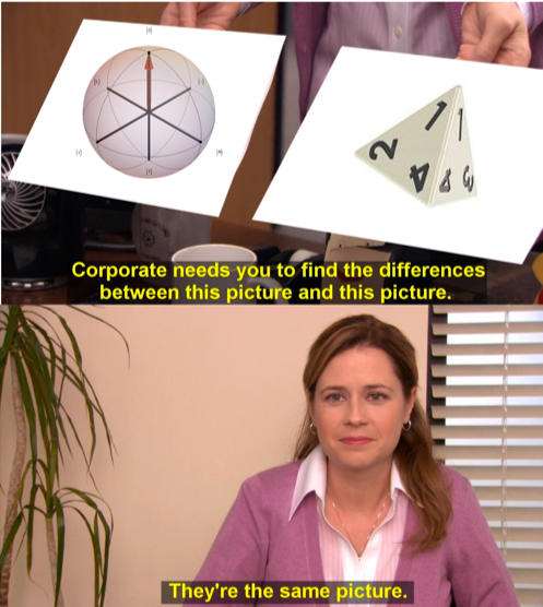
It is called a Tetrahedron because its basis elements form a tetrahedron inside a Bloch sphere:
In[]:=
Simplify@Normalize[QuantumState[First@Eigenvectors@#]["BlochVector"]]&/@QuditBasis["Tetrahedron"]["Elements"]
Out[]=
{0,0,1},-,-,-,-,,-,,0,-
2
3
2
3
1
3
2
3
2
3
1
3
2
2
3
1
3
In[]:=
PolyhedronCoordinates@Tetrahedron2//Simplify
2
3
Out[]=
{0,0,1},-,-,-,-,,-,,0,-
2
3
2
3
1
3
2
3
2
3
1
3
2
2
3
1
3
Out[]=

But if a qubit can be represented by a 4-dimensional probability vector, it means that it belongs to a 3-dimensional simplex embedded in four dimensions:
Every probability vector lies in this simplex:
For a qubit it’s not the case that it maps to an arbitrary probability distribution. Because linear transformation can’t deform a sphere to a simplex. Therefore qubits only occupy a sphere inscribed in that simplex. And strictly speaking as it is a 3-dimensional hyperball embedded in 4D, the Bloch ball (including interior of mixed states) is just a convenient projection we use to visualize it.
Which means that every pure state has the same distance to the hyperball center equal to its radius:
In general hyperball radius has the following dependency on the dimension:
A familiar geometric interpretation of unitary quantum processes taking the form of Bloch sphere rotations now has an immediate generalization of rotating hyperspheres inscribed in probability simplices.
So now we come to the point of asking the obvious question, why not rotate a disk instead?
As an immediate bonus, no projection from 4D to 3D is necessary anymore, as we can easily visualize 2D simplex together with its inscribed disk in its original 3-dimensional space:
This disk represents the probability space of a squtrit. There is no longer a Hilbert space alternative to it, no unitary complex matrices, amplitudes, or phases, but in this doubled space, it still makes perfect sense, and all the analogies from its 4D counterpart can be naturally carried out here as well.
Squtrit states are 3-dimensional probability distributions constrained to a disk inscribed in a simplex triangle. Unitary transformations are rotations (or even reflections, which usually are not considered in conventional quantum computing).
It is now clear why quantum states are constrained to a sphere because otherwise, states can escape a simplex after rotation and would no longer represent valid probabilities and contain negative probabilities instead:
Familiar stochastic maps or Conditional Probability Tables (CPTs), widely used in classical probability theory, are not rotations, they’re combinations of a rotation with a contraction or scaling down of the simplex:
In other words, CPTs always decrease the volume of the simplex. This means that the rotations making up quantum theories can be decomposed into CPTs and an inverse contraction or expansion to preserve the probability space volume of a hyperball.
This expansion is what makes quantum theories special. It is the source of all negative probabilities permeating them and a reason for their computational complexity over classical probability theory.
It doesn’t mean, though, that classical probability lacks this mechanism completely. In fact, it is very common in statistics and takes the form of the famous Bayes rule. It’s the inverse of the predictive contractive process of CPTs, shrinking the space towards a completely uniform mixture in the center. It expands uninformative prior to a larger and more certain posterior, retrodicting it with a stream of observations.
This expansion is what makes quantum theories special. It is the source of all negative probabilities permeating them and a reason for their computational complexity over classical probability theory.
It doesn’t mean, though, that classical probability lacks this mechanism completely. In fact, it is very common in statistics and takes the form of the famous Bayes rule. It’s the inverse of the predictive contractive process of CPTs, shrinking the space towards a completely uniform mixture in the center. It expands uninformative prior to a larger and more certain posterior, retrodicting it with a stream of observations.
Any rotation of a simplex is a Quasi CPT containing negative probabilities satisfying normalization condition:
Rotation can be decomposed into conventional CPT and an expansion controlled by the maximum negative probability as a shrinking parameter:
Expansion doesn’t even provide any new information over CPT alone, as the shrinking parameter is already stored in its inherent orientation and can be extracted using its singular values or its determinant:
Shrinking map is also a valid CPT:
Shrinking is a convex map or a simple weighted average of its input with the uniform distribution in the center:
(In the Bayes rule shrinking map is taking place of the likelihood term)
Expansion on the other hand is a convex-like map with weights still adding up to 1, but which instead assigns a large weight to its input and negative weight to the center:
This expansion map is the cause of all the trouble with trying to simulate quantum computation on a classical computer. While a predictive CPT map can be trivially simulated by resampling with corresponding conditional probabilities to get samples from the resulting distribution, it is not very useful as a computation, given its shrinking behavior. Multiple CPT processes would necessarily shrink the space arbitrarily close to its center and make it indistinguishable from noise. The power of quantum computation comes from preserving the probability space volume while distributions are manipulated in some complex way.
Two squbits can be rotated in 4D, like qubits do, with an additional 3rd degree of freedom being correlation between them. Making a familiar qubit an instance of two correlated biased coins:
With the geometry of two uncorrelated squbits forming a subset inside a Bloch ball in the shape of a potato chip:
It is also obvious that simplex is diffeomorphic to a hyperball; therefore, in principle, it is possible to perform computations with all possible probability distributions after mapping them to a ball, rotating, and mapping back. Here is a corresponding simplex (its 3D projection) and how it morphs into the Bloch sphere:
On the other hand, for quantum computation it is not known how to efficiently progress through its operators in such a linear fashion, as they effectively require keeping track of additional samples at each gate to counteract the noise required to expand probability space back to its original volume. Because of this, quantum circuits are capable of encoding arbitrary distributions in a similarly efficient manner, but from each, it is much harder to sample well-desired outcomes.
All it takes to simulate quantum computation is to blow up a tiny, almost uniform distribution produced by a stochastic part of the circuit to the size of its encompassing hyperball. It may sound straightforward geometrically, but it takes work to do in practice, thanks to the curse of dimensionality.
But in principle, there may be methods of doing it more efficiently with some advanced modern MCMC sampling techniques or even building specific hardware based on molecular and DNA computing to simulate the vast amount of statistical complexity required to probabilistically mimic quantum states and operations on them. It could even give quantum hardware a run for its money by delaying the mythical elusive quantum advantage or perhaps making it ultimately obsolete.
CITE THIS NOTEBOOK
CITE THIS NOTEBOOK
Quantum probability space: geometry of qudits and their square roots
by Nikolay Murzin
Wolfram Community, STAFF PICKS, March 7, 2024
https://community.wolfram.com/groups/-/m/t/3136748
by Nikolay Murzin
Wolfram Community, STAFF PICKS, March 7, 2024
https://community.wolfram.com/groups/-/m/t/3136748