1 | What Is Quantum Computation?
1
| What Is Quantum Computation?Welcome to the first lesson of this course. We start by briefly revisiting classical computation through clear, hands-on examples, then shift to the quantum realm where you will explore a few foundational quantum circuits. Each example comes with accompanying code; if it does not all make sense right away, that's expected — as we progress, you will gradually build both your understanding of quantum concepts and your coding skills.
Key Concepts
Key Concepts
◼
Quantum circuit
◼
Qubit
◼
Measurement
◼
Superposition
◼
Computational basis
Classical Computation
Classical Computation
In order to understand quantum computation, it helps to compare it to classical computation. To compute something, you have to be able to use rules to determine the output from a list of inputs. You can think of computing as starting with the inputs and following the rules to reach an output.
Consider two binary numbers and , and let's see how we can add them. First, each bit-string is interpreted as a base-2 number rather than ordinary decimal, so becomes one and becomes two.
"01"
"10"
"01"
"10"
Define the binary strings:
In[]:=
a="01";b="10";
Construct the number from the base-2 digits of :
a
In[]:=
FromDigits[a,2]
Out[]=
1
Construct the number from the base-2 digits of :
b
In[]:=
FromDigits[b,2]
Out[]=
2
Add the numbers with ordinary addition:
In[]:=
FromDigits[a,2]+FromDigits[b,2]
Out[]=
3
Convert the total back into a bit-string:
In[]:=
IntegerString[FromDigits[a,2]+FromDigits[b,2],2]
Out[]=
11
Now let's add two binary strings and :
"101"
"011"
In[]:=
a="101";b="011";IntegerString[FromDigits[a,2]+FromDigits[b,2],2]
Out[]=
1000
Pay attention to the string length of the initial numbers and the final total. The original bit-strings have length 3, but the answer is a four-bit string. Let's dive in a bit more.
What are all the states of a sequence of three classical bits?
In[]:=
threeBits=Tuples[{0,1},3]
Out[]=
{{0,0,0},{0,0,1},{0,1,0},{0,1,1},{1,0,0},{1,0,1},{1,1,0},{1,1,1}}
What are the corresponding numbers from those base-2 digits?
In[]:=
FromDigits[#,2]&/@threeBits
Out[]=
{0,1,2,3,4,5,6,7}
With a 3-bit string you can represent –; in general, bits represent to -1. Adding and gives 8, which exceeds the 3-bit range. This means in-place addition is modulo , so the sum wraps to unless you provide an extra bit to capture the carry.
0
7
n
0
n
2
101
011
n
2
000
If you stay within 3 bits, perform all operations modulo 8 (wrap-around arithmetic):
In[]:=
Mod[FromDigits[a,2]+FromDigits[b,2],2^3]
Out[]=
0
Then the 3-bit string of that result is:
In[]:=
IntegerString[0,2,3]
Out[]=
000
It is also possible to encode information in such sequences of classical bits to represent problems of interest. For example, each of those bit sequences could also encode a letter character:
In[]:=
FromLetterNumber[FromDigits[#,2]]&/@threeBits
Out[]=
{ ,a,b,c,d,e,f,g}
With yet another encoding scheme, those same bit sequences could represent colors with opacity:
In[]:=
Apply[RGBColor,#]&/@threeBits
Out[]=
,,,,,,,
Having seen how a 3-bit register cleanly enumerates eight distinct states and how different encodings map those states to numbers, letters, or colors, we now move to the quantum setting. There the same eight basis strings exist, but a 3-qubit register can also occupy complex superpositions of them, and even entangled combinations that have no classical analogue. The rules for storing and extracting information therefore change: measurement reveals a single basis outcome, while computation exploits interference among amplitudes.
Quantum Circuits and Qubits
Quantum Circuits and Qubits
Now we dive directly into quantum computation. We introduce common terms and concepts widely used in quantum information. Some details are only briefly mentioned; for each topic we highlight what to focus on for a first exposure, and later we return to expand on each concept in more depth.
The diagram below represents an example of a quantum circuit:
In[]:=
qc=QuantumCircuitOperator[{"H","Z"->2,"Y"->3,"P"[Pi/4],"CNOT"->{1,3},"RY"[Pi/3]->2,"CH"->{2,3},Range[3]}];qc["Diagram"]
Out[]=
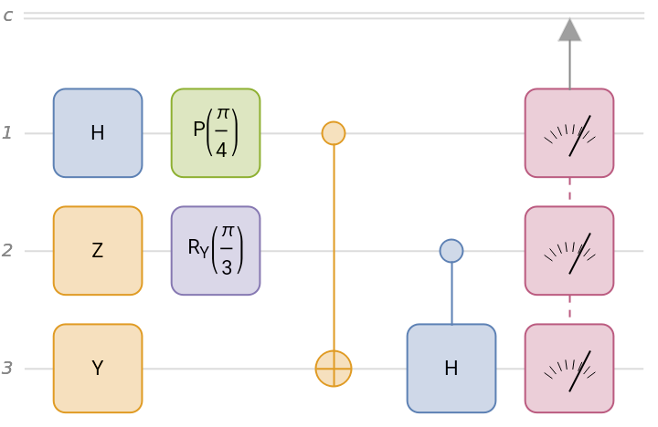
Notice how the circuit diagram has several wires, labeled , , and . Wires , and represent qubits (quantum bits) instead of classical bits. This is a 3-qubit system, meaning that the state can be described in the complex vector space . The previous eight classical bits can form a convenient basis (usually called the computational basis). Those 3-bits in quantum are represented by wrapping them around a notation which is called a ket. In general, a ket is a shorthand representation of a complex-valued vector. A general 3-qubit state is a complex linear combination of those eight basis states.
c
1
2
3
1
2
3
8
C
Ket[{…}]
A quantum circuit is read from left to right. The first operation — represented by the blue box labeled H — acts only on the first wire, while some operations act on more than one wire; they are multi-qubit gates. The boxes that look like gauges on the right represent measurement and point to the wire labeled . The wire labeled represents a classical system (such as part of a regular computer) where the results of the measurements on qubits are stored. All operations shown except measurements are unitary and reversible, a key feature we explore in more detail later. You can think of each box as performing a transformation on the quantum state of one or more wires. These transformations must obey fundamental principles dictated by quantum theory.
c
c
What are the results of running this circuit? Since measurements are included at the end, executing the circuit returns a quantum measurement object in the Wolfram Quantum Framework. This object contains the probability distribution over possible bitstrings and can be sampled to generate measurement outcomes:
In[]:=
measurements=qc[]
Out[]=
QuantumMeasurement

Note that by executing the code above we performed a quantum computation — but it was carried out on a classical computer (your PC). This is exactly what a quantum simulator does: it mimics quantum behavior and performs computations using the rules of quantum mechanics, all within classical hardware.
What are the results of the measurement in this circuit?
In[]:=
measurements["ProbabilitiesPlot"]
Out[]=
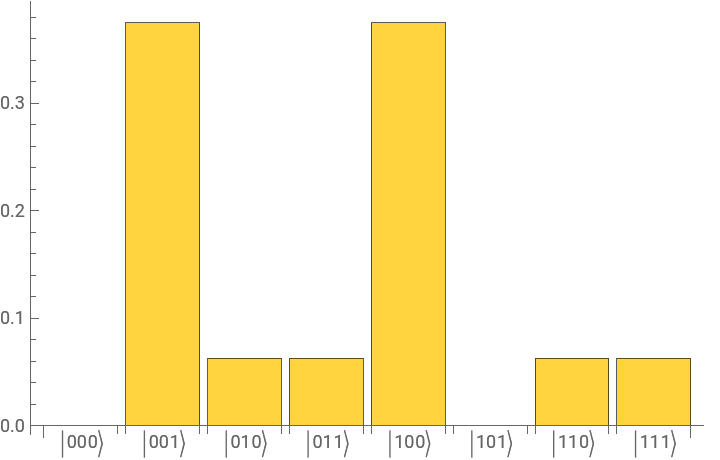
Notice that the possible outcomes of a quantum measurement are simply classical bit sequences. In the earlier classical computation examples, the rules were deterministic: each input led to a definite output. In contrast, quantum computation typically yields a range of possible outcomes, each with a certain probability. This is because quantum theory provides a probabilistic description of measurement results, with the distribution determined by the state just before measurement (and the chosen measurement basis).
For a quantum program to be useful, you arrange things so that the probability of measuring a result that encodes a desired solution to your problem is high.
Additionally, you can track how the quantum state evolves as gates are applied. Although we have not yet discussed the state in full detail, for now focus on the linear combination of computational-basis bitstrings and examine the amplitude of each term. These amplitudes update linearly under gates, and their squared magnitudes determine the probabilities of the corresponding bitstrings upon measurement.
In[]:=
Grid[Prepend[Transpose[{{"Initial","H","Z","Y","P[π/4]","CNOT","RY[π/3]","CH","Measurements"},TraditionalForm/@FoldList[#2[#1]&,QuantumState["000"],qc["Operators"]]}],Style[#,Bold]&/@{"Step","State"}],Frame->All,Alignment->Left]
Out[]=
Step | State |
Initial | |000〉 |
H | 1 2 1 2 |
Z | 1 2 1 2 |
Y | 2 2 |
P[π/4] | 2 π 4 2 |
CNOT | 2 π 4 2 |
RY[π/3] | 1 2 3 2 2 2 1 2 3 2 π 4 π 4 2 2 |
CH | 1 2 3 2 4 4 1 2 3 2 π 4 1 4 π 4 1 4 π 4 |
Measurements | 0000,001 3 8 1 16 1 16 3 8 1 16 1 16 |
Keep in mind that, in the end, the most important information we extract from a quantum system is its measurement results (and their statistics). We will discuss this in more detail in future chapters.
Counting outcomes in a small circuit. Apply a Hadamard to a single qubit in the register state, then measure in the computational basis. What is the probability of each outcome?
Vocabulary
Exercises
Solution
Solution
Solution
The circuit produces an equal superposition and then measures, so the outcomes should be roughly 50/50.
Q&A
Why does the same quantum circuit not always return the same answer?
Quantum measurement is intrinsically probabilistic. Unless the pre-measurement state happens to coincide with one of the measurement basis states, the outcome is drawn from a distribution determined by the state's amplitudes. Repeating the circuit (often called shots) lets you estimate that distribution.
Is the simulator doing real quantum mechanics or just bookkeeping?
Bookkeeping — but the bookkeeping follows the exact rules of quantum theory. The simulator carries the full state vector (or density matrix) and applies the gates as linear operators on a classical computer. A real quantum processor produces the same probability distribution physically; the simulator computes that distribution numerically.
Tech Notes
More to Explore
Summary
In this chapter you saw how classical bits are interpreted as base-2 digits, encoded as numbers, letters, or colors, and saw the bit-width constraint that forces in-place addition to be modular. We then introduced the quantum analogue:
A quantum circuit is a sequence of unitary operations and (optionally) measurements applied to one or more qubits.
A qubit's state is a complex linear combination of the computational basis states, and the squared amplitude of each basis term is the probability of obtaining that bitstring on measurement.
Measurement in the computational basis returns a classical bitstring; the distribution of outcomes is what carries the result of a quantum computation.
A quantum simulator computes the rules of quantum theory on classical hardware, so the output bitstrings have the same statistics as a real quantum processor would produce.
References
M. A. Nielsen and I. L. Chuang, Quantum Computation and Quantum Information, 10th Anniversary Edition, Cambridge University Press, 2010.
S. Aaronson, Quantum Computing Since Democritus, Cambridge University Press, 2013.
Wolfram Research, Wolfram Quantum Framework, paclet documentation, accessed 2026. <https://www.wolfr.am/DevWQCF>
Initialization
Initialization
Install the Wolfram Quantum Framework:
In this chapter we review the common procedure for a quantum algorithm: a state is prepared, some quantum operations are applied, and then measurements are taken. We show how this is captured in an object called a quantum circuit. Along the way we introduce the supporting concepts of quantum state, quantum operator, and quantum basis, and we explore the geometric picture of one-qubit states given by the Bloch sphere.
Key Concepts
Key Concepts
◼
Quantum state
◼
Register state
◼
Quantum operator
◼
Bloch sphere
◼
Computational basis
◼
Bra-ket notation
Quantum Operations
Quantum Operations
Let's consider a generic quantum circuit:
Let's read this circuit step by step (some details may be unfamiliar; we will return to them later):
◼
Qubit 1 is measured in the computational basis.
In classical computation, we use rules to map input states to output states. Quantum operators serve a similar role: they are the rules that transform one quantum state into another. Unlike classical rules, however, they must obey specific constraints set by the formalism of quantum mechanics; in particular, they are linear and (apart from measurements and noise channels) unitary. In the language of quantum computing you will often hear these operators described as "gates" or "gate operations" — terminology borrowed from classical computer engineering.
Quantum States
Quantum States
Quantum states behave differently. When a quantum state is measured, the outcome is always a definite classical result — but the act of measurement inevitably changes the state, a phenomenon known as state collapse. Unlike classical states, quantum states can exist in superpositions. Still, there are special quantum states called computational basis states that always yield the same classical result when measured. These states can be labeled directly by a classical bit string.
If quantum operators in a circuit diagram are the instructions for changing a state, what do we assume about the input state? By convention, most quantum circuit diagrams begin with the register state — the special basis state that always yields the classical result of all zeros when the qubits are measured.
The one-qubit register state can be written as follows:
The Wolfram Quantum Framework returns a summary box for quantum objects because it is much more convenient in practice. Unless the system is very small, other notations — such as full Dirac expressions — are not especially useful for everyday work.
The traditional form of a quantum state returns the conventional Dirac notation:
The above state can be written in different equivalent ways:
Check they are the same:
The two-qubit register state can be written like this:
And so on:
We will discuss quantum states in much more detail in the following chapters. For now, let's focus on different visualizations of a state, without diving deeply into their full meaning.
Bloch Sphere
Bloch Sphere
Since qubits are not the same as classical bits, labeling them by classical bit sequences is insufficient to represent all possible qubit states. How then are quantum states represented?
Future lessons will discuss representing quantum states in more detail. In fact, much of the formalism of quantum mechanics is an important application of linear algebra. However, there is a very useful graphical representation of one-qubit states called the Bloch sphere, named after physicist Felix Bloch.
In this approach a quantum state is represented by a point in 3D space inside a sphere of radius 1 (the Bloch sphere). The point may lie on the surface, in which case we call it a pure state, or inside the sphere, in which case we call it a mixed state.
When thinking about the state of a qubit, you can view it in several equivalent ways:
◼
As a linear combination (a complex-valued 2-vector) in the computational basis.
Generate different representations of a random state:
Bra-Ket Notation
Bra-Ket Notation
In the formalism of quantum mechanics, how to represent and write down the various concepts is an important question. For some common quantum operations, bra-ket notation is particularly useful. This is also sometimes called Dirac notation after P. A. M. Dirac.
Show the matrix form and the Dirac notation of the NOT gate:
Show the Dirac notation of the controlled-Hadamard gate:
Effects of Operations on Qubits
Effects of Operations on Qubits
Consider the following circuit:
The gate labeled "H" is called a Hadamard gate, named after the French mathematician Jacques Salomon Hadamard.
A Quick Note on Measurement
A Quick Note on Measurement
You might wonder at what point probabilities enter the picture. Does the Hadamard gate introduce the need for probability, or does the measurement? Before answering, what happens if a different measurement is performed — one with a special relationship to the Hadamard?
Probability is only necessary when the quantum state before measurement is not in the same basis as the measurement being performed. If you want precise details about this feature of quantum mechanics, it is typically expressed in terms of eigenvalues and eigenvectors of matrices, which you can learn about in a course on linear algebra.
More Operations on Qubits
More Operations on Qubits
Proof
Vocabulary
Exercises
Solution
Solution
Bell-state correlations. Run the Bell-state circuit with 200 shots and tally the bitstring outcomes. What proportion of shots show qubit 1 and qubit 2 with the same value?
Solution
Q&A
Why does the Hadamard gate not introduce randomness on its own?
The Hadamard gate is a unitary operation — it deterministically transforms a definite quantum state into another definite quantum state. The randomness only appears when you measure; the measurement basis decides whether the resulting state lies along a definite axis (deterministic outcome) or sits at some angle to it (probabilistic outcome).
Tech Notes
More to Explore
Summary
This chapter introduced the basic building blocks of quantum circuits and the surrounding language:
The Bloch sphere is a 3D geometric representation of a single qubit's state: pure states lie on the surface, mixed states inside.
Bra-ket notation is a compact way to write quantum states (kets) and their conjugates (bras); composite states are tensor products of single-qubit kets.
Measurement outcomes are probabilistic in general, but a state that aligns with the measurement basis yields a deterministic outcome.
References
M. A. Nielsen and I. L. Chuang, Quantum Computation and Quantum Information, 10th Anniversary Edition, Cambridge University Press, 2010, Chapters 1–2.
J. Preskill, Lecture Notes on Quantum Computation, Caltech, accessed 2026. <http://theory.caltech.edu/~preskill/ph229/>
F. Bloch, "Nuclear Induction", Physical Review 70, 460 (1946).
Initialization
Initialization