2 | Building Blocks of Quantum Circuits
2
| Building Blocks of Quantum CircuitsIn this chapter we review the common procedure for a quantum algorithm: a state is prepared, some quantum operations are applied, and then measurements are taken. We show how this is captured in an object called a quantum circuit. Along the way we introduce the supporting concepts of quantum state, quantum operator, and quantum basis, and we explore the geometric picture of one-qubit states given by the Bloch sphere.
Key Concepts
Key Concepts
◼
Quantum state
◼
Register state
◼
Quantum operator
◼
Bloch sphere
◼
Computational basis
◼
Bra-ket notation
Quantum Operations
Quantum Operations
Let's consider a generic quantum circuit:
In[]:=
QuantumCircuitOperator[{"H","S"->2,"C"["RY"[Pi/3]]->{1,2},"C"["NOT"->2,{},{1}],"BitFlip","SWAP",{1}}]["Diagram"]
Out[]=
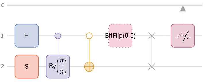
Let's read this circuit step by step (some details may be unfamiliar; we will return to them later):
◼
Since no initial state is given, the two qubits are prepared in the register state .
Ket[{00}]
◼
A Hadamard gate acts on qubit 1.
H
◼
An gate acts on qubit 2.
S
◼
A conditional rotation about by angle acts on both qubits: if qubit 1 is in state , apply the rotation on qubit 2; otherwise do nothing.
Y
π/3
Ket[{1}]
◼
A conditional-0 acts on both qubits: if qubit 1 is in state , apply an () to qubit 2; otherwise do nothing.
NOT
Ket[{0}]
X
NOT
◼
A bit-flip noise channel acts on qubit 1 with rate .
1/2
◼
A gate acts on both qubits.
SWAP
◼
Qubit 1 is measured in the computational basis.
In classical computation, we use rules to map input states to output states. Quantum operators serve a similar role: they are the rules that transform one quantum state into another. Unlike classical rules, however, they must obey specific constraints set by the formalism of quantum mechanics; in particular, they are linear and (apart from measurements and noise channels) unitary. In the language of quantum computing you will often hear these operators described as "gates" or "gate operations" — terminology borrowed from classical computer engineering.
Quantum States
Quantum States
In classical digital computing, states are represented by sequences of s and s. Each classical bit has two possible states, or . A sequence of two bits has four possible states: , , , or . In general, a sequence of classical bits has possible states.
1
0
0
1
"00"
"01"
"10"
"11"
n
n
2
Quantum states behave differently. When a quantum state is measured, the outcome is always a definite classical result — but the act of measurement inevitably changes the state, a phenomenon known as state collapse. Unlike classical states, quantum states can exist in superpositions. Still, there are special quantum states called computational basis states that always yield the same classical result when measured. These states can be labeled directly by a classical bit string.
If quantum operators in a circuit diagram are the instructions for changing a state, what do we assume about the input state? By convention, most quantum circuit diagrams begin with the register state — the special basis state that always yields the classical result of all zeros when the qubits are measured.
The one-qubit register state can be written as follows:
In[]:=
QuantumState["Register"]
Out[]=
QuantumState
The Wolfram Quantum Framework returns a summary box for quantum objects because it is much more convenient in practice. Unless the system is very small, other notations — such as full Dirac expressions — are not especially useful for everyday work.
The traditional form of a quantum state returns the conventional Dirac notation:
In[]:=
QuantumState["Register"]//TraditionalForm
Out[]=
|0〉
The above state can be written in different equivalent ways:
In[]:=
QuantumState["0"]
Out[]=
QuantumState
Check they are the same:
In[]:=
QuantumState["Register"]==QuantumState["0"]
Out[]=
True
The two-qubit register state can be written like this:
In[]:=
QuantumState["Register"[2]]//TraditionalForm
Out[]=
|00〉
And so on:
In[]:=
TraditionalForm/@Table[QuantumState["Register"[n]],{n,3,6}]
Out[]=
{,,,}
|000〉
|0000〉
|00000〉
|000000〉
Throughout this course we follow the big-endian (usual Dirac) convention, as opposed to the little-endian (usual IBM) convention. In big-endian, a state such as means qubit-1 is in the state and qubit-2 is in the state .
Ket[{01}]
Ket[{0}]
Ket[{1}]
A register state is shorthand for a unit vector of length whose first element is one and all others are zero:
Ket[{0^⊗n}]
n
2
In[]:=
Table["n="<>ToString[n]->Normal@QuantumState[StringJoin@ConstantArray["0",n]]["StateVector"],{n,5}]//Column
Out[]=
n=1{1,0} |
n=2{1,0,0,0} |
n=3{1,0,0,0,0,0,0,0} |
n=4{1,0,0,0,0,0,0,0,0,0,0,0,0,0,0,0} |
n=5{1,0,0,0,0,0,0,0,0,0,0,0,0,0,0,0,0,0,0,0,0,0,0,0,0,0,0,0,0,0,0,0} |
We will discuss quantum states in much more detail in the following chapters. For now, let's focus on different visualizations of a state, without diving deeply into their full meaning.
Bloch Sphere
Bloch Sphere
Since qubits are not the same as classical bits, labeling them by classical bit sequences is insufficient to represent all possible qubit states. How then are quantum states represented?
Future lessons will discuss representing quantum states in more detail. In fact, much of the formalism of quantum mechanics is an important application of linear algebra. However, there is a very useful graphical representation of one-qubit states called the Bloch sphere, named after physicist Felix Bloch.
In this approach a quantum state is represented by a point in 3D space inside a sphere of radius 1 (the Bloch sphere). The point may lie on the surface, in which case we call it a pure state, or inside the sphere, in which case we call it a mixed state.
Compute the Bloch vector of :
Ket[{0}]
In[]:=
QuantumState["0"]["BlochVector"]
Out[]=
{0,0,1}
The Bloch sphere representation of the qubit state :
Ket[{0}]
In[]:=
QuantumState["0"]["BlochPlot"]
Out[]=

Compute the Bloch vector of :
Ket[{1}]
In[]:=
QuantumState["1"]["BlochVector"]
Out[]=
{0,0,-1}
Notice that the qubit state is on the opposite side of the sphere from .
Ket[{1}]
Ket[{0}]
In[]:=
QuantumState["1"]["BlochPlot"]
Out[]=

When thinking about the state of a qubit, you can view it in several equivalent ways:
◼
As a linear combination (a complex-valued 2-vector) in the computational basis.
Generate different representations of a random state:
Bra-Ket Notation
Bra-Ket Notation
In the formalism of quantum mechanics, how to represent and write down the various concepts is an important question. For some common quantum operations, bra-ket notation is particularly useful. This is also sometimes called Dirac notation after P. A. M. Dirac.
Show the matrix form and the Dirac notation of the NOT gate:
Show the Dirac notation of the controlled-Hadamard gate:
Effects of Operations on Qubits
Effects of Operations on Qubits
Consider the following circuit:
The gate labeled "H" is called a Hadamard gate, named after the French mathematician Jacques Salomon Hadamard.
A Quick Note on Measurement
A Quick Note on Measurement
You might wonder at what point probabilities enter the picture. Does the Hadamard gate introduce the need for probability, or does the measurement? Before answering, what happens if a different measurement is performed — one with a special relationship to the Hadamard?
Probability is only necessary when the quantum state before measurement is not in the same basis as the measurement being performed. If you want precise details about this feature of quantum mechanics, it is typically expressed in terms of eigenvalues and eigenvectors of matrices, which you can learn about in a course on linear algebra.
More Operations on Qubits
More Operations on Qubits
Proof
Vocabulary
Exercises
Solution
Solution
Bell-state correlations. Run the Bell-state circuit with 200 shots and tally the bitstring outcomes. What proportion of shots show qubit 1 and qubit 2 with the same value?
Solution
Q&A
Why does the Hadamard gate not introduce randomness on its own?
The Hadamard gate is a unitary operation — it deterministically transforms a definite quantum state into another definite quantum state. The randomness only appears when you measure; the measurement basis decides whether the resulting state lies along a definite axis (deterministic outcome) or sits at some angle to it (probabilistic outcome).
Tech Notes
More to Explore
Summary
This chapter introduced the basic building blocks of quantum circuits and the surrounding language:
The Bloch sphere is a 3D geometric representation of a single qubit's state: pure states lie on the surface, mixed states inside.
Bra-ket notation is a compact way to write quantum states (kets) and their conjugates (bras); composite states are tensor products of single-qubit kets.
Measurement outcomes are probabilistic in general, but a state that aligns with the measurement basis yields a deterministic outcome.
References
M. A. Nielsen and I. L. Chuang, Quantum Computation and Quantum Information, 10th Anniversary Edition, Cambridge University Press, 2010, Chapters 1–2.
J. Preskill, Lecture Notes on Quantum Computation, Caltech, accessed 2026. <http://theory.caltech.edu/~preskill/ph229/>
F. Bloch, "Nuclear Induction", Physical Review 70, 460 (1946).
Initialization
Initialization