Discrete-Time Quantum Walk on a Line
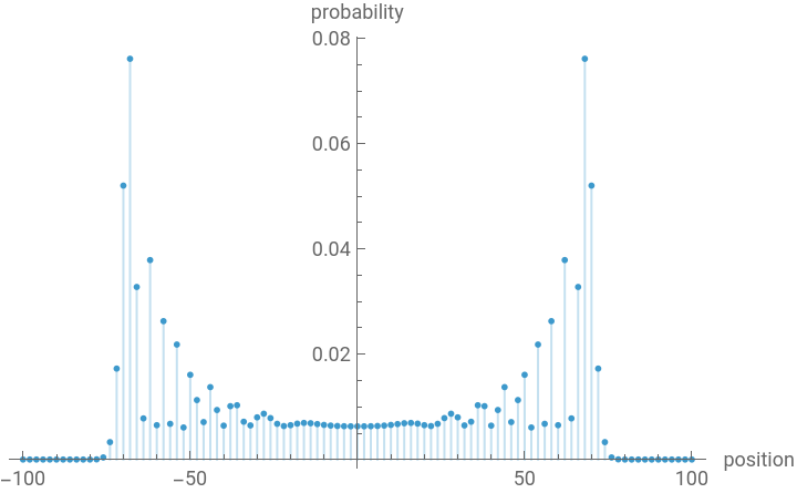
After 100 steps the distribution has two sharp peaks near , far from the origin where a classical walker would concentrate. Only same-parity sites are occupied at each step, so plot every other site:
±𝑛/
2
In[1]:=
points[p_]:=Transpose[{Range[-100,100],p}][[1;;;;2]];distribution=Last[quantumWalk[100]];ListPlot[points[distribution],Filling->Axis,PlotRange->All,AxesLabel->{"position","probability"}]
Out[1]=
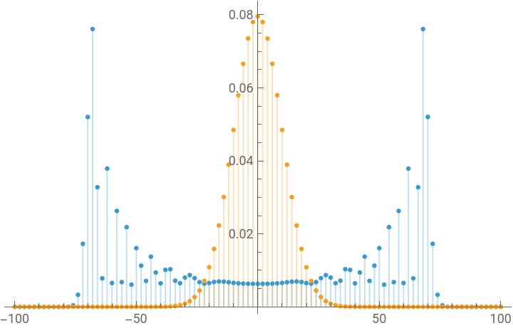
The classical random walk of the same length is a binomial distribution: a single Gaussian peak at the origin. Overlaying the two shows ballistic versus diffusive transport:
In[2]:=
classical=Table[If[EvenQ[x],Binomial[100,(x+100)/2]/2^100,0],{x,-100,100}];ListPlot[{points[distribution],points[classical]},Filling->Axis,PlotRange->All,PlotLegends->{"quantum","classical"}]
Out[2]=


_________________________________________________________________________________________________________________
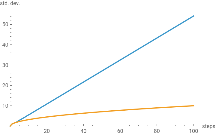
The spreading rates differ qualitatively: the quantum standard deviation grows linearly in the number of steps, while the classical one grows like :
𝑡
In[1]:=
sites=Range[-100,100];spread[p_]:=Sqrt[p.sites^2-(p.sites)^2];evolution=quantumWalk[100];ListLinePlot[{Table[{t,spread[evolution[[t+1]]]},{t,0,100}],Table[{t,Sqrt[t]},{t,0,100}]},PlotLegends->{"quantum (~ t)","classical (~ Sqrt[t])"},AxesLabel->{"steps","std. dev."}]
Out[1]=