Sophisticated time series functions automatically select from built-in fitting methods for highly accurate forecasting, with options for creating and fitting new classes of hybrid models.
Examples in Multiparadigm Data Science:
Time Series
Examples in Multiparadigm Data Science:
Time Series
Time Series
Use TimeSeriesModelFit to create seasonal autoregressive integrated moving-average process (SARIMA)
models in a few lines of code.
models in a few lines of code.
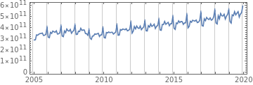
Model seasonal data of monthly retail sales in the United States. Begin by querying Wolfram|Alpha:
raw=WolframAlpha["usa retail sales",{{"History:RetailSales:EconomicData",1},"TimeSeriesData"}];
data=TimeSeries[{QuantityMagnitude[raw[[-12*15;;,2]]]},{Automatic,raw[[-1,1]],"Month"}];grids=Table[{1992,12i},{i,data["PathLength"]}];DateListPlot[data,GridLines{grids,None},AspectRatio1/3]
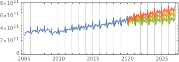
Fit a seasonal model and generate process parameters using TimeSeriesModelFit and forecast the
next seven years with 95% confidence bands:
next seven years with 95% confidence bands:
model=TimeSeriesModelFit[data,{"SARIMA",12}];proc=model["BestFit"];forecast=TimeSeriesForecast[model,{0,7*12}];α=.95;q=Quantile[NormalDistribution[],1-(1-α)/2];err=forecast["MeanSquaredErrors"];bands=TimeSeriesThread[{{1,-q}.#,{1,q}.#}&,{forecast,Sqrt[err]}];grids=Table[{1992,12i},{i,data["PathLength"]+forecast["PathLength"]}];DateListPlot[{data,forecast,bands["PathComponent",1],bands["PathComponent",2]},Filling{3{4}},AspectRatio1/3,PlotStyleAutomatic,GridLines{grids,None}]
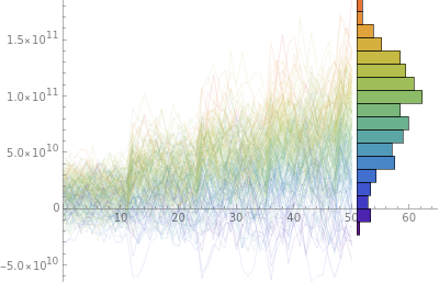
rfproc=RandomFunction[proc,{50},200];sd=rfproc["SliceData",50];cf=ColorData["Rainbow"];sliced=BarChart[Last[#],AxesFalse,BarOriginLeft,AspectRatio4,ChartStyle(cf/@Rescale[MovingAverage[First[#],2],{Min[sd],Max[sd]},{0,1}]),ImageSize65]&[HistogramList[sd,{Range[Min[sd],Max[sd],(Max[sd]-Min[sd])/20]}]];ListLinePlot[rfproc,ImageSize400,PlotRangeAll,AspectRatio3/4,EpilogInset[sliced,{51,0},{0,2.5}],PlotStyle(cf/@Rescale[sd]),BaseStyleDirective[Thin,Opacity[0.5]],PlotRangePadding{{0,15},{.5,.5}}]
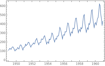
Fit a time series model and forecast airline passenger volume using ExampleData. Obtain the monthly
total number of US international airline passengers (in thousands) from January 1949 to December 1960:
total number of US international airline passengers (in thousands) from January 1949 to December 1960:
passengers=ExampleData[{"Statistics","InternationalAirlinePassengers"},"TimeSeries"]
TimeSeries

Make a simple plot to examine the data:
DateListPlot[passengers,JoinedTrue]
tsm=TimeSeriesModelFit[passengers,{"SARIMA",12}]
TimeSeriesModel
proc=tsm["Process"]
SARIMAProcess[0.22472,{-0.361058},1,{},{12,{-0.128311,0.234166},1,{}},130.919]
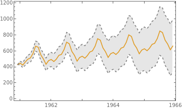
Forecast for the next five years with a plot of prediction bands:
k=5;start="December 1st, 1960";forecastDates=DateRange[start,DatePlus[start,{k,"Year"}],"Month"];forecast=tsm/@forecastDates;bands=tsm["PredictionLimits"][#]&/@forecastDates;pforecast=DateListPlot[{bands[[All,1]],forecast,bands[[All,2]]},{start,Automatic,"Month"},JoinedTrue,Filling{1{3}},PlotStyle{Directive[{Dashed,Gray}],Automatic,Directive[{Dashed,Gray}]}]
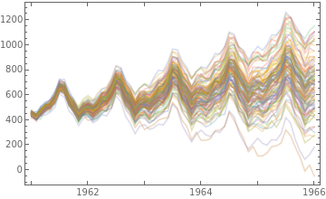
Simulate the next five years:
k=5;sim=RandomFunction[tsm,{0,12*k},100];psim=DateListPlot[sim,PlotStyleDirective[Opacity[.25]],JoinedTrue,PlotRangeAll]
Find the mean function of the simulated paths and make a plot:
Go Further:
Go Further: