In[]:=
f_samp=10^3;(*samplingfrequency[Hz]*)
In[]:=
T_samp=1/f_samp;(*samplingperiod[s]*)
In[]:=
T_gate=10;(*gatetime[sec]*)
N_samp=T_gate*f_samp(*thenumberofthesamples*)
Out[]=
10000
In[]:=
σ=1;
In[]:=
samples=RandomVariate[NormalDistribution[0,σ],N_samp]+I*RandomVariate[NormalDistribution[0,σ],N_samp];
In[]:=
DTFT[T_,ω_,data_]:=Sum[data[[n]]*Exp[-I*ω*T*n],{n,Length[data]}]
In[]:=
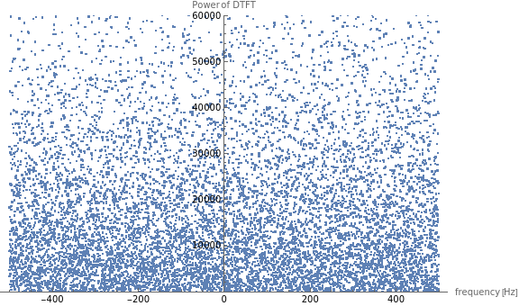
Block[{res_f=0.1(*resolutionoff*)},spectrum=ParallelTable[DTFT[T_samp,2Pi*f,samples],{f,-f_samp/2,f_samp/2,res_f}];ListPlot[Re[Conjugate[spectrum]*spectrum],DataRange{-f_samp/2,f_samp/2},AxesLabel{"frequency [Hz]","Power of DTFT"},PlotRange{0,3*2N_samp*σ^2},ImageSizeLarge]]

Out[]=
Block[{plt1,plt2},plt1=Histogram[Re[Conjugate[spectrum]*spectrum]/(N_samp*σ^2),{0,8,0.1},"CDF",ChartLegends{"simulation"}];plt2=Plot[CDF[ChiSquareDistribution[2],x],{x,0,8},PlotLegends{"ideal CDF"}];Show[plt1,plt2]]
Out[]=