166: 6.1 Example 5
166: 6.1 Example 5
Example 5(a): Estimating the Net Distance and Total Distance Traveled When Velocity is Given as a Function:
Example 5(a): Estimating the Net Distance and Total Distance Traveled When Velocity is Given as a Function:
Using the Fundamental Theorem of Calculus (Part 2), we see that if we are given a rate function f '(t), such as velocity, then the change in the corresponding amount function, in this case position, from t=a to t=b is given by f'(t)t. For example, if we know that our velocity is given by v(t) = s '(t) = + 3 t miles/hour for times t≥0 hours, then the net distance in miles traveled between times t=1 and t=3 hours is:
b
∫
a
3
t
In[]:=
v[t_]:=t^3+3t
Integrate[v[t],{t,1,3}]
Out[]=
32
Thus, the net distance traveled is 8.25 miles.
Plot[v[t],{t,1,3},PlotLabel->"v(t) velocity (miles/ hour)",AxesLabel->{t,"v(t)"},PlotRange->{0,40},Filling->Axis]
Out[]=
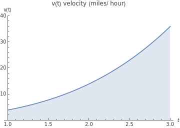
Since the graph of v(t) lies entirely above the t-axis on the t-interval [1, 3], the total distance traveled is equal to the net distance traveled.
Example 5(b): Estimating the Net Distance and Total Distance Traveled When the Velocity is Given as a Graph:
Example 5(b): Estimating the Net Distance and Total Distance Traveled When the Velocity is Given as a Graph:
Suppose our velocity function is given by the function , and we don’t know the distance function s(t) such that . We can still estimate the net distance and total distance traveled by looking at the area trapped between the graph of the velocity function and the t-axis.
v(t)=t*sin(t)
s'(t)=v(t)
In[]:=
Clear[v]
In[]:=
v[t_]:=t*Sin[t]
Plot[v[t],{t,0,8},PlotRange->{-10,10},PlotLabel->"v(t) velocity (miles/ hour)",AxesLabel->{t,"v(t)"},Filling->Axis,FillingStyle->{LightRed,LightBlue}]
Out[]=

On the t-interval [0, 8], the net distance traveled is the signed area, i.e the area above the t-axis (light blue) minus red area below the t-axis (light red). One way to estimate the signed area is via Riemann sums. Let’s use n equal subintervals from [a, b] = [0, 8], of width , and for sample point choose the midpoint of each subinterval, =a+*Δt.
Δt===1
(b-a)
n
(8-0)
8
t
i
t
i
(2i-1)
2
In[]:=
a=0;b=8;deltat[n_]:=(b-a)/n
deltat[8]
Out[]=
1
Table of velocity values at each midpoint:
TableForm[Table[{i,a+(2i-1)/2*deltat[8],v[a+(2i-1)/2*deltat[8]]},{i,1,8}],TableHeadings->{None,{"i","t_i","v[t_i]"}}]
Out[]//TableForm=
i | t_i | v[t_i] |
1 | 1 2 | 1 2 1 2 |
2 | 3 2 | 3 2 3 2 |
3 | 5 2 | 5 2 5 2 |
4 | 7 2 | 7 2 7 2 |
5 | 9 2 | 9 2 9 2 |
6 | 11 2 | 11 2 11 2 |
7 | 13 2 | 13 2 13 2 |
8 | 15 2 | 15 2 15 2 |
Numerical values of table entries:
TableForm[Table[{i,a+(2i-1)/2*deltat[8],v[a+(2i-1)/2*deltat[8]]},{i,1,8}],TableHeadings->{None,{"i","t_i","v[t_i]"}}]//N
Out[]//TableForm=
i | t_i | v[t_i] |
1. | 0.5 | 0.239713 |
2. | 1.5 | 1.49624 |
3. | 2.5 | 1.49618 |
4. | 3.5 | -1.22774 |
5. | 4.5 | -4.39889 |
6. | 5.5 | -3.88047 |
7. | 6.5 | 1.39828 |
8. | 7.5 | 7.035 |
Riemann sum estimate of net distance traveled:
Sum[v[a+(2i-1)/2*deltat[8]]*deltat[8],{i,1,8}]
Out[]=
1
2
1
2
3
2
3
2
5
2
5
2
7
2
7
2
9
2
9
2
11
2
11
2
13
2
13
2
15
2
15
2
N[%]
Out[]=
2.15832
Thus the approximate net distance traveled is 2.15832 miles.
Here is a graphical comparison of the rectangles used in the Riemann sum estimate to the graph of v(t):
In[]:=
nceiling[x_,n_]:=Ceiling[n*x]/n
In[]:=
nfloor[x_,n_]:=Floor[n*x]/n
Show[{Plot[v[1/2(nfloor[t,1]+nceiling[t,1])],{t,0,8},PlotRange->{-10,10},PlotLabel->"v(t) velocity (miles/ hour)",AxesLabel->{t,"v(t)"},Filling->Axis,FillingStyle->{LightRed,LightBlue}],Plot[v[t],{t,0,8},PlotRange->{-10,10}]}]
Out[]=
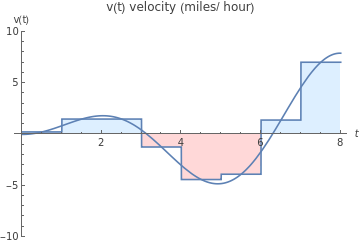
To get a better approximation, use more rectangles in the Riemann sum. Letting n = 20, 50, 100, and 500, we get the following approximate net distances traveled :
TableForm[Table[{n,Sum[v[a+(2i-1.)/2*deltat[n]]*deltat[n],{i,1,n}]},{n,{20,50,200,500}}],TableHeadings->{None,{"n","Riemann Sum Estimate"}}]
Out[]//TableForm=
n | Riemann Sum Estimate |
20 | 2.15447 |
50 | 2.15354 |
200 | 2.15337 |
500 | 2.15336 |
To find the total distance traveled, we need to find the total area trapped between the graph of y = v(t) and the t-axis.
Plot[v[t],{t,0,8},PlotRange->{-10,10},PlotLabel->"v(t) velocity (miles/ hour)",AxesLabel->{t,"v(t)"},Filling->Axis,FillingStyle->{LightRed,LightBlue},Ticks->{{{3.13,"t1"},{6.28,"t2"},{8,"8"}},Automatic}]
Out[]=
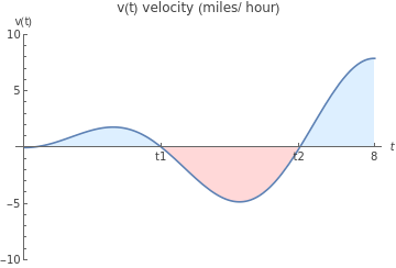
Table of absolute value of velocity values at each midpoint:
Numerical values of table entries:
Riemann sum estimate of total distance traveled:
Here is a graphical comparison of the rectangles used in the Riemann sum estimate to the graph of |v(t)|: