The properties of a Leontief production function in the TLO model

Parameters

In[]:=

Clear[a1,a2,b1,b2]

In[]:=

a1=0.1;a2=0.1;b1=0.1;b2=0.3;

The standard Leontief model

◼

Assumes fixed input requirements

◼

Assume output of y requires a1 units of input w and a2 units of input c

◼

Can be formulated mathematically using Min. function

In[]:=

y[w_,c_]:=Min[a1w,a2c]

◼

The properties of this production function are well-known and straightforward to establish.

◼

In terms of linearity;

◼

it is linear to scale expansion and displays constant returns to scale;

◼

its level sets (isoquants) are piecewise linear.

◼

Min[ . ] is fundamentally a non-linear function; in particular its continuous but not differentiable

◼

To draw smooth surfaces we use a differentiable approximation to the the Min. function

In[]:=

ya[w_,c_]:=-

Log

(Exp[-ρa1w]+Exp[-ρa2c])

In[]:=

ρ=100;Print["The approximation for w = 10, c = 5"]ya[10,5]//NPrint["The exact Leontief"]y[10,5]

The approximation for w = 10, c = 5

Out[]=

0.506931

The exact Leontief

Out[]=

0.5

◼

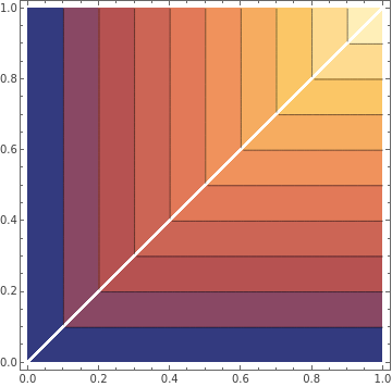
Here are exact and approximations compared graphically

In[]:=

{Plot3D[y[a,b],{a,0,1},{b,0,1}],Plot3D[ya[a,b],{a,0,1},{b,0,1}]}

Out[]=





In[]:=

{ContourPlot[y[a,b],{a,0,1},{b,0,1}],ContourPlot[ya[a,b],{a,0,1},{b,0,1}]}

Out[]=





◼

By making the approximation closer ρ  ∞ the piecewise linearity is nearly preserved. And there will always be constant returns to scale.

◼

I wish to examine these two aspects of linearity (scale and isoquants) as we generalise the function in ways that accord with the implementation inTLO model has many outputs (treatments) and has stochastic elements generating the requirements for treatments.

Multi-output Leontief

◼

The requirement to produce another output is analogous to an adjustment to the inputs available to produce the first output.

◼

Here is a deterministic Leontief production function with the output y1 as a function of two inputs and an output y2

In[]:=

y1[w_,c_,y2_]:=Min[a1(w-b1y2),a2(c-b2y2)]

With y2 = 0 the functions and the diagrams above apply

Scale linearity with non-zero y2

◼

The second output is analogous to negative set of inputs - i.e. its presence reduces available inputs for y1.

◼

If we just fix that output and scale up inputs we get increasing returns to scale in respect of y1.

◼

Explanation ; the degrading effect on inputs gets smaller as the inputs gets larger. We can just see that with some numerical examples.

In[]:=

y1[10,50,0]

Out[]=

In[]:=

y1[20,100,0]

Out[]=

◼

With zero y2 we have constant returns as expected

◼

With positive y2

In[]:=

y1[10,50,10]

Out[]=

0.9

In[]:=

y1[20,100,10]

Out[]=

1.9

◼

So output has increased by a factor of

In[]:=

y1[20,100,10]/y1[10,50,10]

Out[]=

2.11111

◼

Hence increasing returns

◼

If we doubled output 2 at the same time as doubling inputs ....

In[]:=

y1[20,100,40]/y1[10,50,20]

Out[]=

In[]:=

y1[20,100,20]==2y1[10,50,10]

Out[]=

True

◼

Back to constant returns to scale.

Isoquants

◼

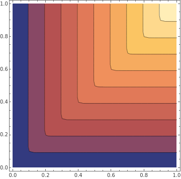
The piecewise linearity of isoquants is preserved. Varying the additional output just shifts the isoquants.

In[]:=

Plot3D[y1[a,b,0],{a,0,1},{b,0,1}]

Out[]=

In[]:=

zeroy2=ContourPlot[y1[a,b,0],{a,0,1},{b,0,1}]

Out[]=

In[]:=

Export["/Users/martinchalkley/Desktop/upload/fig2a.png",zeroy2]

◼

With output y2.

◼

The resulting contour plot.

What does the production function for y1 look like ‘on average’ - as y2 varies

◼

If we were to use the TLO model to empirically estimate the production function y1[ ] what would the resulting function look like.

◼

That is to say we look at model outputs (number of treatments y1, as the inputs are varied)

◼

The model will be generating varying demands on the health system from y2. But if we average over lots of those model simulations, first for given level of inputs w and c, and then repeated the exercise for lots of different values of w and c what would we expect to see?

y2 as a random variable

◼

Now let y2 by a random variable say Uniform on 0, 1

◼

We are interested in the expectation of output and we notice something interesting in terms of non-linearity of this expectation

◼

Because Min is a non linear function, its expectation is not equal to expected value of y2, and this process of taking expectations removes the piecewise linearity of isoquants.

What about returns to scale - in this expected sense

◼

Now we are averaging over a given range of values for y2 - and therefore not linking y2 to the scaling of inputs, the idea we explored above replicates itself. We will have non-constant (actually increasing) returns to scale.

Generalise this to two other outputs

◼

We know the model has lots of other outputs. We can expect that this will further ‘non-linearise’ the production function.

◼

Here is an example -

◼

First, some input requirement parameters for a second additional output.

◼

The generalisation of the stochastic case depends on the relationship between the two other outputs. If they are independent the we use the multivariate uniform - i.e. pdf = 1

◼

From here on it makes sense to do discrete plots as the time taken for Plot3D becomes problematic. This steps involved are create a table of data:

◼

The plots can be made smoother

◼

The deviation from piecewise linear is greater - subjectively these are looking like isoquants of a more standard production function that displays diminishing marginal rates of substitution between inputs.

Interdependent other outputs

◼

Handling the case of not independently distributed rvs is more challenging.

◼

Here I continue to consider bivariate uniform on 0,1 and consider copulas as a means of capturing interdependency.

◼

I use the Ali-Mikhail-Haq copula because it is analytically simple.

◼

There is a single parameter θ ∈ (-1,1) - that determines the interdependency (θ = 0  independence)

◼

Checking the formulation here -- integrating this over u gives the marginal density for for u,

Indefinite integral

◼

Which is independent of u

◼

To get the joint pdf

◼

Again - a further shift from linearity.

Conclusion

◼

Even a simple an apparently linear “Leontief” production function will generate a rich non-linear set of production relationships in the context of the TLO model.

Martin Chalkley