Symbolic vs numeric computation
Symbolic vs numeric computation
By now, we’ve learned just a few algebraic tricks for integration:
◼
u
◼
Integration by parts, and
◼
application of those to trig functions.
There are plenty more techniques that get more and more specific. In this document, though, we’re going to focus on how to ask a computer algebra system to do integrals for us. While we’ll discuss both symbolic and numeric integration, we’ll ultimately focus on numerics and why they’re so important.
In this document, we’ll be using Mathematica, mainly because it’s widely regarded as the most powerful commercial system for computer algebra, has excellent tools for both symbolics and numerics, and because UNCA has a site licence that gives us easy access.
In this document, we’ll be using Mathematica, mainly because it’s widely regarded as the most powerful commercial system for computer algebra, has excellent tools for both symbolics and numerics, and because UNCA has a site licence that gives us easy access.
Symbolic vs Numeric computation for solving equations
Symbolic vs Numeric computation for solving equations
Here’s an example of a symbolic computation:
In[]:=
Solve[x^2-20,x]
Out[]=
{x-
2
},{x2
}Here’s a very similar, but numeric computation:
In[]:=
NSolve[x^2-20,x]
Out[]=
{{x-1.41421},{x1.41421}}
In[]:=
%//InputForm
Out[]//InputForm=
{{x -> -1.4142135623730951}, {x -> 1.414213562373095}}
See the difference? Symbolic computations are exact, while numeric computations yield decimal approximations. The symbolic solution indeed yields exactly 0 when we plug it into our equation:
2
In[]:=
2
2
Out[]=
0
But the decimal approximation misses by a bit:
In[]:=
2
1.414213562373095
Out[]=
-4.44089×
-16
10
Symbolic and numeric algorithms are very different. Obviously, exact symbolic exact solutions have their advantages. Numeric algorithms tend to be much easier to implement, much faster, and more generally applicable. For example, here’s a very innocent looking equation that Solve can’t seem to solve:
In[]:=
Solve[Cos[x]x,x]

Out[]=
Solve[Cos[x]x,x]
But, the numeric FindRoot command has no problem:
In[]:=
FindRoot[Cos[x]x,{x,1}]
Out[]=
{x0.739085}
We can look at the problem geometrically to ensure that this looks good.
In[]:=
Plot[{Cos[x],x},{x,0,1.2},Epilog{PointSize[Large],Point[{0.739,0.739}]}]
Out[]=
Even when Solve works, the output can be very complicated - almost incomprehensible:
In[]:=
Solve[-x-10,x]
3
x
Out[]=
x,x,x
In[]:=
%//ToRadicals
Out[]=
x-+,x-(1---,x-(1+--
1
3
1/3
27
2
3
69
2
1/3
(9+
1
2
69
)2/3
3
1
6
3
)1/3
27
2
3
69
2
(1+
3
)1/3
(9+
1
2
69
)2
2/3
3
1
6
3
)1/3
27
2
3
69
2
(1-
3
)1/3
(9+
1
2
69
)2
2/3
3
But NSolve expresses all the roots in a simple format
In[]:=
NSolve[-x-10,x]
3
x
Out[]=
{{x-0.662359-0.56228},{x-0.662359+0.56228},{x1.32472}}
In[]:=
%//ToRadicals
Out[]=
{{x-0.662359-0.56228},{x-0.662359+0.56228},{x1.32472}}
Integration
Integration
Integration can also be performed symbolically or numerically. Symbolically, we can do an indefinite integral:
In[]:=
Integrate[x^2-x-1,x]
Out[]=
-x-+
2
x
2
3
x
3
Or a definite integral:
In[]:=
Integrate[x^2-x-1,{x,0,2}]
Out[]=
-
4
3
There’s no numeric analog to an indefinite integral but there is to a definite integral:
In[]:=
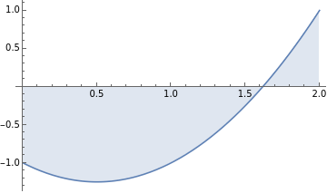
NIntegrate[x^2-x-1,{x,0,2}]
Out[]=
-1.33333
Geometrically, this number should represent the “signed” area we see here:
In[]:=
Plot[x^2-x-1,{x,0,2},FillingAxis]
Out[]=
Of course, Mathematica can do much harder functions:
In[]:=
Integrate516+4Cos+20-+Cos+Sin+Sin[x],x
4x
-4+4x
4x
2+4x
4x
4x
4x
-4
4x
4x
4x
4x
Out[]=
-5+5Cos-Cos[x]+5+4xSin
-4+4x
4x
4x
4x
4x
4x
But there are, again, quite innocent expressions that Mathematica cannot integrate:
In[]:=
Integrate[Sin[Cos[x]],x]
Out[]=
∫Sin[Cos[x]]x
Though, it might give some kinda crazy answer for a definite integral:
In[]:=
Integrate[Sin[Cos[x]],{x,0,Pi/2}]
Out[]=
1
2
NIntegrate returns a more palatable response for a numeric integral
In[]:=
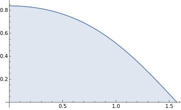
NIntegrate[Sin[Cos[x]],{x,0,Pi/2}]
Out[]=
0.893244
That looks reasonable
In[]:=
Plot[Sin[Cos[x]],{x,0,Pi/2},FillingAxis]
Out[]=
Special functions
Special functions
Here’s a function whose integral is very important in statistics:
In[]:=
f[x_]=
1
2π
-2
2
x
This is the standard, normal distribution or so-called bell curve:
The funny constant in front is chosen so that total area under the curve is 1:
While Mathematica knows the exact value of this specific definite integral, the indefinite integral is expresses the antiderivative in terms of a mysterious symbol called Erf.
And most definite integrals are expressed in terms of Erf as well.
So what is Erf??
If you read the documentation more closely, you’ll find that Erf is literally defined to be
So, Erf is really just a placeholder name representing the integral that we were looking for in the first place.
As it turns out, the normal distribution can be used to compute all sorts of probabilities. For example, if we generate a number with a standard normal distribution, the probability that it lies between plus or minus one is about 68%, according to the following calculation:
Key Points
Key Points
We’ll talk more about this function later in the semester. The key points to digest at the moment are
◼
There are simply expressed functions that don’t have any simply expressed antiderivative,
◼
Such functions often arise in applied mathematics, and
◼
There are numerical techniques for computing definite integrals associated with these functions.