Fourier Series - continuous periodic signals
Fourier Series - continuous periodic signals
Fourier Trigonometrical Series
Fourier Trigonometrical Series
Introduction to Fourier Trigonometrical Series
Introduction to Fourier Trigonometrical Series
A continuous periodic signal x(t) with period T, meeting the Dirichlet conditions, can be represented by the infinite sum of harmonics:
with:
- are even spectrum coefficients for n=0,1,2,3,... (,,stand next to cosines'')
- are odd spectrum coefficients for, n=1,2,3,... (,,stand next to sines'')
Dirichlet conditions
If the following conditions hold:
1. f must be absolutely integrable over a period:
2. f must be of bounded variation in any given bounded interval.
3. f must have a finite number of discontinuities in any given bounded interval, and the discontinuities cannot be infinite.
Then we can reresent f with a Fourier series.
Example of a Fourier series for x(t)=|t| in interval <-π,π> (so T=2π), for n=5 (this does not mean that there are five parts).
In[]:=
FourierTrigSeries[t , t, 3]
Out[]=
2Sin[t]-Sin[2t]+Sin[3t]
2
3
Below options of FourierTrigSeries[]: default the interval is <-π,π>
In[]:=
Options[FourierTrigSeries]
Out[]=
{Assumptions$Assumptions,FourierParameters{1,1},GenerateConditionsFalse}
FourierTrigSeries[Abs[t],t,7,FourierParameters{1,Pi}](*inrange<-1,1>*)
Out[]=
1
2
4Cos[πt]
2
π
4Cos[3πt]
9
2
π
4Cos[5πt]
25
2
π
4Cos[7πt]
49
2
π
In[]:=
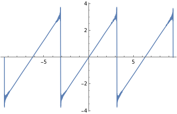
Plot[Evaluate[FourierTrigSeries[t,t,200]],{t,-3Pi,3Pi}]
Out[]=
In[]:=
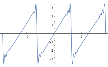
Plot[Evaluate[FourierTrigSeries[t,t,15]],{t,-3Pi,3Pi}]
Out[]=
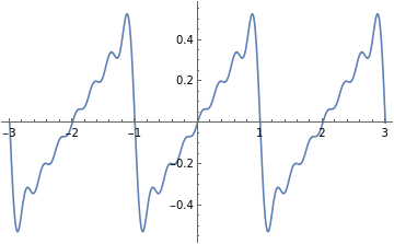
Below, a function expansion in Fourier series in the range <-1,1>. Change of FourierParameters {0, Pi}
In[]:=
Plot[Evaluate[FourierTrigSeries[t,t,7,FourierParameters{0,Pi}]],{t,-3,3}]
Out[]=
Some Plot[] options:
In[]:=
Options[Plot]
In[]:=
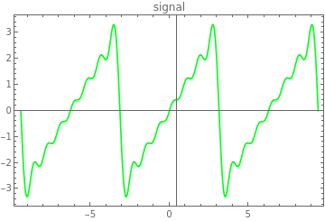
f[x_]:=FourierTrigSeries[x,x,7]Plot[Evaluate[f[t]],{t,-3Pi,3Pi},FrameTrue,PlotRangeAll,PlotLabel"signal",AxesOrigin{0.5,0},PlotStyleHue[0.35]]
Out[]=
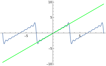
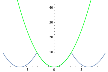
The following are: functions - in green, expansions in Fourier series of these functions in interval <-π, π> - in blue:
In[]:=
Show[Plot[Evaluate[FourierTrigSeries[x,x,10]],{x,-3Pi,3Pi},PlotRangeAll],Plot[x,{x,-3Pi,3Pi},PlotRangeAll,PlotStyleHue[0.35]]]Show[Plot[Evaluate[FourierTrigSeries[x^2,x,10]],{x,-3Pi,3Pi},PlotRange{0,45}],Plot[x^2,{x,-3Pi,3Pi},PlotRangeAll,PlotStyleHue[0.35]]]Show[Plot[Evaluate[FourierTrigSeries[Abs[x]+x,x,10]],{x,-3Pi,3Pi},PlotRangeAll],Plot[Abs[x]+x,{x,-3Pi,3Pi},PlotRangeAll,PlotStyleHue[0.35]]]
Out[]=
Out[]=
Out[]=

Examples: sawtooth-shaped, rectangular, triangular signal
Examples: sawtooth-shaped, rectangular, triangular signal
Examples: even and odd signals
Examples: even and odd signals