Using Computation and Analysis for Business Insights
5
|Choose a Location for the Company
Introduction
When selecting a location for a business, especially in a remote market, factors like population, average home value or climate might impact the decision. Can we use computation to research and compare cities to find a city with a large population and low average home value?
Wolfram Curated Data for US Cities
Wolfram Curated Data for US Cities
Wolfram Language has built-in data for cities that can be accessed with a single command called CityData. The following calculation returns the population for Key West, Florida:
In[]:=
CityData[{"Key West","Florida","UnitedStates"},"Population"]
Out[]=
CityData also includes some precomputed terms to help filter data. Using the term returns all cities in the state of Florida with a population over 100,000:
Large
In[]:=
cities=CityData[{Large,"Florida","UnitedStates"}]
Out[]=
,,,,,,,,,,,,,,,,,,,,,,,,,
The orange icons are called Entities in Wolfram Language and indicate there is more data available for that particular city. The Entity representation of a city in Wolfram Language gives us an easy way to query other factors, like population or median home value for a particular city:
In[]:=
Out[]=
Out[]=
To compare the cities, we can create a table of values using the list of cities above. The extra set of curly brackets in the following calculation is used to group related values together. In the following calculation, Table first assigns the city Seattle to the symbol and then returns that city name, the population for Seattle and the median home value for Seattle in a list. Table then assigns the city Spokane to the symbol and returns the same three results for that city. Table repeats the process for all nine cities. The result is a list with two sets of curly brackets; you can think of this like a spreadsheet with nine rows and three columns of data:
c
c
In[]:=
results=Table[{c,c["Population"],c["MedianHomeValue"]},{c,cities}]
Out[]=
,,,,,,,,,,,,,,,,,,,,,,,,,,,,,,,,,,,,,,,,,,,,,,,,,,,,,,,,,,,,,,,,,,,,,,,,,,,,,
Based on a quick scan through the data, you might already notice Lakeland is the best fit based on the original goals. But a sorted grid of values might be useful for a presentation. Wolfram Language also includes functions to sort data, like Sort or SortBy, as well as functions like TextGrid to display data in a nice grid so it’s easy to read:
In[]:=
TextGrid[SortBy[results,Last],Frame->All]
Out[]=
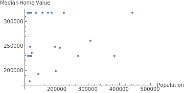
In addition to a table of values, Wolfram Language has many built-in commands to create charts or plots. ListPlot creates a scatter plot. The Part command can extract rows and then the second and third columns in the symbol result to give us the data for the scatter plot. Both ListPlot and TextGrid in the last calculation include additional options to customize the result. The option used above draws the spreadsheet-like frame around the result. The option draws labels on the and axes to make the scatter plot more descriptive. Both are optional, and the commands work without those additional options:
All
Frame
AxesLabel
x
y
In[]:=
ListPlot[Part[results,All,{2,3}],AxesLabel->{"Population","Median Home Value"}]
Out[]=
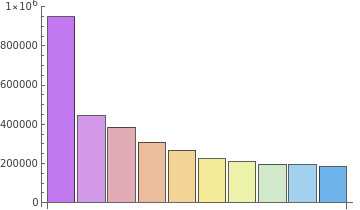
A bar chart might also be useful to visualize just the population data for the largest 10 cities. Part can be used to return the first through the tenth rows, along with the second column in the list stored with the symbol name result:
In[]:=
BarChart[Part[results,1;;10,2],ChartLegends->Part[results,1;;10,1],ChartStyle->"Pastel"]
Out[]=
Summary
Summary
It is often possible to get data on cities from websites or other data sources. But the curated data in Wolfram Language is a nice way to work with the data all in one structured environment and easily visualize aspects of the data.