9 | Eigenvalues and eigenvectors
9 | Eigenvalues and eigenvectors
This chapter of Linear Algebra by Dr JH Klopper is licensed under an Attribution-NonCommercial-NoDerivatives 4.0 International Licence available at http://creativecommons.org/licenses/by-nc-nd/4.0/?ref=chooser-v1 .
9.1 Introduction
9.1 Introduction
In this notebook we investigate interesting matrices that act as operators on vectors.
9.2 Eigenvalues
9.2 Eigenvalues
Definition 9.2.1 Consider a square matrix and a non-zero vector . We define as an eigenvector of if the following property holds, shown in (1).
A
n×n
v∈
n
v
A
Av=λv
(
1
)Definition 9.2.1 Here is a scalar, , multiple of . This scalar, , is the eigenvalue of of and is the eigenvector of corresponding to .
Av
λ
v
λ
A
v
A
λ
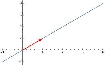
Below, we have a line through the origin and a vector, on that line.
v=(1,2)
In[]:=
Show[Plot[2x,{x,-1,4}],Graphics[{Red,Thick,Arrow[{{0,0},{1,2}}]}]]
Out[]=
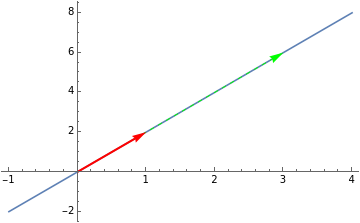
In (2) we have a matrix .
A
A=
3 | 0 |
8 | -1 |
(
2
)Note the result of the multiplication of this matrix and the vector, .
v
In[]:=
A={{3,0},{8,-1}};v={1,2};MatrixForm[A.v]
Out[]//MatrixForm=
3 |
6 |
In the plot below, we see that the result is a scalar multiple of . Indeed we have . It is still on the same line and is just a scalar multiple of .
v
Av=3v
v
In[]:=
Show[Plot[2x,{x,-1,4}],Graphics[{Green,Dashed,Arrow[{{0,0},{3,6}}]}],Graphics[{Red,Thick,Arrow[{{0,0},{1,2}}]}]]
Out[]=
Multiplying an identity matrix of appropriate dimension with a vector returns the same vector. We can therefor, do the following manipulation, shown in (3).
Av=λIvλIv-Av=0(λI-A)v=0
(
3
)Since we chose to be a non-zero vector, the only way for (3) to hold is for the determinant of to be , shown in (4).
v
λI-A
0
|λI-A|=0
(
4
)Equation (4) is known as the characteristic equation of . This result is always a polynomial known as the characteristic polynomial of , shown in (5).
A
A
n
λ
c
1
n-1
λ
c
n
(
5
)As an example, we have the (6).
λI=λ
=
,A=
λI-A=
|λI-A|=[(λ-1)(λ-4)]-(2)(3)=0-5λ-2=0
1 | 0 |
0 | 1 |
λ | 0 |
0 | λ |
1 | 2 |
3 | 4 |
λ-1 | 2 |
3 | λ-4 |
2
λ
(
6
)We check on our work using the Det function.
In[]:=
Det[{{λ-1,2},{3,λ-4}}]
Out[]=
-2-5λ+
2
λ
We solve for using the Solve function.
λ
In[]:=
Solve[Det[{{λ-1,2},{3,λ-4}}]0,λ]
Out[]=
λ(5-(5+
1
2
33
),λ1
2
33
)These are the two eigenvalues of . The Eigenvalues function will return the same results.
A
In[]:=
Eigenvalues[{{1,2},{3,4}}]
Out[]=
(5+(5-
1
2
33
),1
2
33
)It is a simple task to calculate the determinant of triangular matrix. It is the product of the entries along the main diagonal. The characteristic polynomial of such an upper triangular matrix is shown in (7).
|A-λI|=
=0(λ-)(λ-)…(λ-)=0
λ- a 11 | - a 12 | ⋯ | - a 1n |
0 | λ- a 22 | ⋯ | - a 2n |
⋮ | ⋮ | ⋱ | ⋮ |
0 | 0 | ⋯ | λ- a nn |
a
11
a
22
a
nn
(
7
)The eigenvalues are then as shown in (8), i.e. the entries along the main diagonal.
λ={,,…,}
a
11
a
22
a
nn
(
8
)As an example we have the lower triangular matrix below.
In[]:=
L={{2,0,0},{3,-1,0},{-1,2,4}};MatrixForm[L]LowerTriangularMatrixQ[L]
Out[]//MatrixForm=
2 | 0 | 0 |
3 | -1 | 0 |
-1 | 2 | 4 |
Out[]=
True
In[]:=
Eigenvalues[L]
Out[]=
{4,2,-1}
It is possible for a matrix to have complex eigenvalues. Consider the matrix below, ().
A=
-3 | -1 |
6 | 1 |
(
9
)The characteristic polynomial of this matrix determines the eigenvalues, ().
=0(λ+3)(λ-1)-(-1)(6)=0+2λ+3=0
λ+3 | -1 |
6 | λ-1 |
2
λ
(
10
)In[]:=
Solve[+2λ+30,λ]
2
λ
Out[]=
{λ-1-
2
},{λ-1+2
}We note the complex roots, with the eigenvalues confirmed using the Eigenvalues function.
In[]:=
Eigenvalues[A]
Out[]=
-1+
2
,-1-2
Some square matrices are not invertible, shown in (11).
A=
3 | 6 |
-2 | -4 |
(
11
)Their determinants are .
0
In[]:=
Det[{{3,6},{-2,-4}}]
Out[]=
0
Their eigenvalues include .
0
In[]:=
Eigenvalues[{{3,6},{-2,-4}}]
Out[]=
{-1,0}
This means that square matrix is invertible if and only it does not have as an eigenvalue.
0
9.3 Eigenvectors
9.3 Eigenvectors
We have seen the definition of an eigenvector of a matrix corresponding to an eigenvalue, . The eigenvectors are then the solutions in the nullspace of that is all the vectors, , such that . This nullspace is called the eigenspace of corresponding to .
A
λ
(λI-A)
v
(λI-A)v=0
A
λ
To calculate the eigenvectors, we need to find a basis for the eigenspace. Consider the example matrix below, shown in (12).
A
A=
0 | 0 | -2 |
1 | 2 | 1 |
1 | 0 | 3 |
(
12
)In[]:=
A={{0,0,-2},{1,2,1},{1,0,3}};Eigenvalues[A]
The basis is calculated below, shown in (13).
9.3.1 Matrix powers
9.3.1 Matrix powers
Note the eigenvalues of this matrix.
9.4 Diagonalization
9.4 Diagonalization
Here we are concerned with finding the basis for a square matrix, such that the basis consists of eigenvectors.
Below, we use code to demonstrate that the result is a diagonal matrix.
Some matrices are not diagonalizable, ().
There are only two eigenvectors (which are non-zero vectors).
This is not to say that matrices with non-distinct eigenvalues are not diagonalizable. Look below at the identity matrix. It is triangular, with three identical eigenvalues.
It has three eigenvectors, though, and is diagonalizable.
One of our previous examples also has repeated eigenvalues, but is diagonalizable.
It is indeed a diagonal matrix. Now we raise it to the fifth power.
9.5 Orthogonal diagonalization
9.5 Orthogonal diagonalization