12 | THE ANTIDERIVATIVE
12 | THE ANTIDERIVATIVE
This chapter of Single Variable Calculus by Dr JH Klopper is licensed under an Attribution-NonCommercial-NoDerivatives 4.0 International Licence available at http://creativecommons.org/licenses/by-nc-nd/4.0/?ref=chooser-v1 .
12.1 Introduction
12.1 Introduction
In the previous chapter we were introduced to the concept of a definite integral and learned that we can use it to calculate the area under the curve on the interval of a function.
The integral is more than just an area though. In this chapter we learn about the fundamental theorem of calculus and see the deep connection between the derivative and the integral.
12.2 Review of the definite integral
12.2 Review of the definite integral
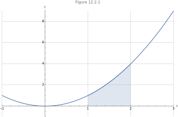
If we consider the function we can use the definite integral to calculate the area between the curve and the axis in a specific interval such as . We write the problem in (1) and then calculate it using the Wolfram Language.
f(x)
2
x
x
[1,2]
2
∫
1
2
x
(
1
)In[]:=
2
∫
1
2
x
Out[]=
7
3
Figure 12.2.1 visualizes the definite integral.
In[]:=
Show[Plot[,{x,-1,3},PlotRange->{{-1,3},{-1,9}},PlotLabel->"Figure 12.2.1",AxesLabel->{"x","y"},GridLines->Automatic,ImageSize->Large],Plot[,{x,1,2},Filling->Axis,PlotRange->{{1,2},{-1,9}}]]
2
x
2
x
Out[]=
12.3 The indefinite integral
12.3 The indefinite integral
We can also consider the integral without specifying the lower and the upper bound of integral. Such as integral is named an indefinite integral.
We see the notation for such an integral in (2).
∫dx
2
x
(
2
)Note that we have not written any numbers for the integration symbol .
∫
To understand the concept of the indefinite integral, we explore the antiderivative.
12.4 The antiderivative
12.4 The antiderivative
Consider the function . We know that the first derivative with respect to this function is (x)2x using the power rule of the derivative.
f(x)
2
x
′
f
Below, we explore the indefinite integral of the expression .
2x
In[]:=
∫2xx
Out[]=
2
x
We note that it is . As a matter of warning, the actual solution is , where is an arbitrary constant, named the constant of integration. More on this later. Many computer languages can can do symbolic integration assumes that we know that we have to always add a constant of integration and does not actually add it to the solution.
2x
2x+c
c
It is interesting though that we started with the function and used its first derivative in the indefinite integral, only to get back to . Below, we consider the polynomial . We create a user-defined function f to hold the function .
f(x)
2
x
2
x
f(x)-2x+1
2
x
f
In[]:=
f[x_]:=-2x+1
2
x
Next, we take the first derivative of with respect to using the D function.
f
x
In[]:=
D[f[x],x]
Out[]=
-2+2x
As expected, using the power rule, we get (x)2x-2. Below, we use this expression in an indefinite integral.
′
f
In[]:=
∫(2x-2)x
Out[]=
-2x+
2
x
Remembering the constant of integration, we have -2x+c. With , this is our initial function .
2
x
c1
f(x)
We can now formalize the relationship between a derivative and an integral. First, though a definition.
Definition 12.4.1 In any integral we name the integrand.
∫f(x)dx
f(x)
If we have an arbitrary function and its first derivate (x)f(x), then we can write (3).
F(x)
′
F
F(x)∫f(x)dx
(
3
)In (3) we see that the integrand of an integral is the first derivative of the solution to the integral. We state that the solution to the integral is the antiderivative. When we integrate, we reverse the process of taking the derivative in some sense.
Fortunately for use, depending on the integrand , there are many analytical processes such as the power rule, the product rule, the quotient rule and many others that we can explore in order to solve integration problems. We start with the power rule of integration.
f(x)
12.5 The power rule of integration
12.5 The power rule of integration
We can use the power rule of integration for any polynomial . We start with a simple polynomial , where is a constant. The indefinite integral using the power rule of integration is shown in (4).
f(x)
f(x)a
n
x
a
adx+c
n
x
a
n+1
n+1
x
(
4
)As an example, we consider . We use the Wolfram Language to calculate the indefinite integral.
f(x)5
2
x
In[]:=
∫5x
2
x
Out[]=
5
3
x
3
As the power rule of integration shows, we have that . We divide the coefficient by and the power of is now also .
2+13
5
3
x
2+13
The complete solution is given in (5).
F(x)+c
5
3
3
x
(
5
)The reason for the constant of integration follows from the fact that is the antiderivative of the integrand . The derivative of a constant is . It does not matter what value the constant stakes. Below, we let and take the first derivative of .
c
F(x)
f(x)
0
c2
F(x)+2
5
3
3
x
In[]:=
D+2,x
5
3
3
x
Out[]=
5
2
x
The solution is the integrand. The solution to an indefinite integral is actually then a family of solutions.
F(x)
Problem 12.5.1 Calculate the indefinite integral .
∫3dx
We can still use the power rule of integration when we realize that . We have that . The solution is calculated below.
33
0
x
0+11
In[]:=
∫3x
Out[]=
3x
The full solution is . This makes sense since (x)3.
F(x)3x+c
′
F
There is an important property of the integration of when consists of terms that are added or subtracted. In (6) we see a polynomial (consisting of three terms) and show that the integral of is the sum of the integral of the terms.
f(x)
f(x)
f(x)
∫-2x+1dx∫dx+∫-2xdx+∫1dx
2
x
2
x
(
6
)We show that the results are similar using the Wolfram Language.
In[]:=
∫(-2x+1)x
2
x
Out[]=
x-+
2
x
3
x
3
In[]:=
∫x+∫(-2x)x+∫1x
2
x
Out[]=
x-+
2
x
3
x
3
Another important property of the integral consider any coefficients. A coefficients is not involved in the integration and we can write the property in (7).
∫af(x)dxa∫f(x)dx
(
7
)As an example we reconsider one of the terms in (6) and that is . We see that the property in (7) holds.
∫-2xdx
In[]:=
∫-2xx
Out[]=
-
2
x
Next we take the coefficient out of the integral.
In[]:=
-2∫xx
Out[]=
-
2
x
The solutions are the same. Remember, though, that the actual solution in . Never forget the constant of integration when writing the solution to an indefinite integral.
-+c
2
x
12.6 The fundamental theorem of calculus
12.6 The fundamental theorem of calculus
We take yet another look at the definite integral. In () we reconsider dx. We can now use the power rule and write ().
2
∫
1
2
x
2
∫
1
2
x
1
3
3
x
x=2
|
x=1
(
8
)We confirm the result using the Wolfram Language.
We can now write the fundamental theorem of calculus.
Theorem 12.6.1 The fundamental theorem of calculus is written as shown in (10).
This is exactly the theorem that we applied in (9).
Problem 12.6.1 Use the fundamental theorem of calculus to determine the definite integral in (11).
Figure 12.6.1 visualizes the problem.
We use the Wolfram Language to confirm the result.
Problem 12.6.2 Calculate the definite integral in (13).
In (14) we use the fundamental theorem of calculus to solve the problem.
We have a negative value as the solution. We confirm the result using the Wolfram Language.
We can also consider definite integrals where the area is both above and below the curve.
Figure 12.6.3 visualizes the problem.
The solution can still be calculated using the fundamental theorem of calculus. We use the Wolfram Language to calculate the solution.
The result is still the same.