11 | INTRODUCTION TO INTEGRATION
11 | INTRODUCTION TO INTEGRATION
This chapter of Single Variable Calculus by Dr JH Klopper is licensed under an Attribution-NonCommercial-NoDerivatives 4.0 International Licence available at http://creativecommons.org/licenses/by-nc-nd/4.0/?ref=chooser-v1 .
11.1 Introduction
11.1 Introduction
Whereas the derivative explained the rate of change, we now move on the understanding the area under a curve of a function. In this chapter we introduced the second topic in calculus, which is integration.
We start by considering the idea of the area of rectangles to build our intuition for the definite integral.
Building this intuition for integration will help us in the next chapter where we have a proper introduction to integration using the anti-derivative and the indefinite integral.
11.2 The area under a curve
11.2 The area under a curve
Consider the curve of the function and, more specifically, the area between the curve and the axis from to , shown as the light blue area in Figure 11.2.1,which is termed the area under the curve.
f(x)
2
x
x
x2
x3
In[]:=
Show[Plot[,{x,-1,4},PlotRange->{{-1,4},{-1,16}},PlotLabel->"Figure 11.2.1",AxesLabel->{"x","y"},GridLines->Automatic,ImageSize->Large],Plot[,{x,2,3},PlotRange->{{2,3},{-1,10}},Filling->Axis]]
2
x
2
x
Out[]=
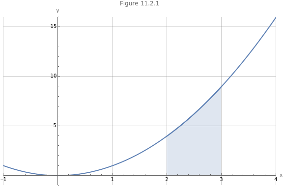
We know the formulae for the areas of squares, rectangles, triangles, circles, and many more shapes. The area under the curve in Figure 11.2.1 does not have a defined formula, though. Instead we develop the idea of integration to calculate this area under the curve.
To develop and understanding of integration, we start to explore the method of Riemann sums.
11.3 Riemann sums method of numerical integration
11.3 Riemann sums method of numerical integration
The Riemann sum method to approximate the integral is the sum of the areas of rectangles formed between the curve and the axis.
x
The area of a rectangle is given in (1), where is the base and is the height.
A
x
y
A=xy
(
1
)We can calculate the height of a rectangle by considering the value of a function at a point , shown in Figure 11.3.1.
(x,f(x))
In[]:=
Show[ListPlot[{{2,}},PlotRange->{{-1,4},{-1,16}},PlotLabel->"Figure 11.3.1",AxesLabel->{"x","y"},GridLines->Automatic,ImageSize->Large],Graphics[{Orange,Thick,Line[{{2,},{3,}}],Line[{{3,0},{3,}}],Line[{{2,0},{2,}}],Line[{{2,0},{3,0}}]}],Plot[,{x,-1,4}]]
2
2
2
2
2
2
2
2
2
2
2
x
Out[]=
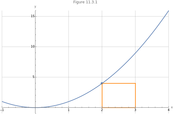
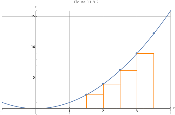
Figure 11.3.1 denotes a left-rectangle as the height of the rectangle is determined at the left-most value of . Figure 11.3.2 shows four such left Riemann rectangles. Note that we can approximate the area under the curve from to by adding all the areas of the rectangles. This is a left Riemann sum.
yf(x)
x
x
start
3
2
x
finish
7
2
In[]:=
ShowListPlot,,{2,},,,{3,},,,PlotRange->{{-1,4},{-1,16}},PlotLabel->"Figure 11.3.2",AxesLabel->{"x","y"},GridLines->Automatic,ImageSize->Large,GraphicsOrange,Thick,Line{3,},,,Line,,3,,Line{2,},,,Line,,2,,Line,0,,,Line[{{3,0},{3,}}],Line[{{2,0},{2,}}],Line,0,,,Line,0,,,Line,0,,0,Plot[,{x,-1,4}]
3
2
2
3
2
2
2
5
2
2
5
2
2
3
7
2
2
7
2
2
(3)
7
2
2
(3)
5
2
2
5
2
2
5
2
2
(2)
5
2
2
(2)
3
2
2
3
2
2
3
2
3
2
3
2
2
3
2
2
3
2
2
5
2
5
2
2
5
2
7
2
7
2
2
(3)
3
2
7
2
2
x
Out[]=
For a step size of a starting value of and an end value of , defining an interval of integration, we calculate sub-intervals, as shown in (2).
h
x
start
x
finish
n
n=-
x
finish
x
start
h
(
2
)In Figure 11.3.2 we start at and end at . For a step size of , we calculate in (3).
x
start
3
2
x
finish
7
2
h
1
2
n
n=-===4
7
2
3
2
1
2
4
2
1
2
2
1
2
(
3
)There are indeed rectangles in Figure 11.3.2. The values of that we require for calculating the height of each rectangle are ,2,, and . This would be +0(h), +1(h), +2(h), and +3(h). For a left Riemann sum we end at added to .
n4
x
3
2
5
2
3
x
start
x
start
x
start
x
start
(n-1)h
x
start
We can sum over all the left Riemann rectangles using (4). Note that we end the summation at -h, which can also be written as +(n-1)h, as is clear from Figure 11.3.2.
x
finish
x
start
hf(x+ih)
n-1
∑
i=0
(
4
)A user-defined function named area can be created from (4), where the parameters x1 is , x2 is , and h is the step size .
x
start
x
finish
h
In[]:=
area[x1_,x2_,h_]:=Modulen=,hf[x1+ih]
x2-x1
h
n-1
∑
i=0
We consider the function and create a user-defined function f to hold our function .
f(x)
2
x
f
In[]:=
f[x_]:=
2
x
We can now use the function area for the interval 1, 5, and a step size .
x
start
x
finish
h0.0001
In[]:=
area[1,5,0.0001]
Out[]=
41.3321
It should be clear that in the case of Figure 11.3.2 that we under-estimate the area under the curve as the sum of the areas of the rectangles are smaller that the actual area under the curve.
Left Riemann sums are not the only way to approximate the area under a curve. We can also use right Riemann sums or even mid-point sums. We can even have different step sizes for each rectangle. The trapezoidal method is another such method that we explore in section 11.5. First, though, we use the idea of a Riemann sum to develop an understanding of the definite integral.
11.4 The definite integral
11.4 The definite integral
We start with a very simple definition of a definite integral.
Definition 11.4.1 A definite integral is the area under the curve of a function on and interval to , where .
f(x)
xa
xb
b>a
We can use the idea of a Riemann sum and limits to develop the understanding the definite integral.
Our step size was set as a constant in section 11.3. Using the Riemann sum we used values of and to determine the area of each rectangle. In essence, we can write (5), where our step size is and we sum over all the sub-intervals . Note that we are approximating the area.
x
yf(x)
hΔx
X
area≈ f(x)Δx
∑
X
(
5
)If there are sub intervals then the area is approximated in (6).
n
area≈f(x)Δx
n
∑
i=1
(
6
)We can make our step size infinitely small and have the number of sub intervals approach infinity. In the limit we write (7).
n
area=f(x)Δx
lim
n->∞
n
∑
i=1
(
7
)From Definition 11.4.1 we name and the bounds of integration. For these bounds, we write the definite integral in (8), which follows from the limit in (7), where we use the integral symbol to replace the infinite summation , and where we have an infinitely small step size .
a
b
∫
Σ
x
In the next section we develop the trapezoidal method of numerical integration which can be more accurate than using the sum of rectangles.
11.5 Trapezoidal method of numerical integration
11.5 Trapezoidal method of numerical integration
The Wolfram Language is used in the code cell below to show the integral.