10 | APPLICATIONS OF THE DERIVATIVE AND NUMERICAL DIFFERENTIATION
10 | APPLICATIONS OF THE DERIVATIVE AND NUMERICAL DIFFERENTIATION
This chapter of Single Variable Calculus by Dr JH Klopper is licensed under an Attribution-NonCommercial-NoDerivatives 4.0 International Licence available at http://creativecommons.org/licenses/by-nc-nd/4.0/?ref=chooser-v1 .
10.1 Introduction
10.1 Introduction
There are many uses and applications for the derivative. This is especially true in the field of health data science, where many of the statistical and machine learning techniques that we use requiring differentiation.
In this chapter we begin with a numerical method for finding the roots of a function. While a typical course in single variable calculus develops techniques for calculating roots exactly, we must sometimes rely on numerical methods.
In the rest of the chapter we explore the use of the derivative in optimization problems. Here, we try and calculate values for an unknown so that we can maximize a specified value. Optimization is used to solve real-world problems.
We also explore how to find the maximum or minimum of a function using the derivative. Deep neural networks use this method to learn from data.
At the end of the chapter we revisit the equation for the derivative and develop numerical methods for calculating a derivative.
10.2 Newton’s method of finding roots
10.2 Newton’s method of finding roots
y-=m(x-)y=m(x-)+
y
0
x
0
x
0
y
0
(
1
)The slope is simply the derivative of the function and is . At the point we have f() and the slope (). We substitute these values into (1) in (2), the equation for the tangent to the function at .
m
yf(x)
m(x)
′
f
x
x
0
y
0
x
0
′
f
x
0
f
(,)
x
0
y
0
y=f'()(x-)+f()
x
0
x
0
x
0
(
2
)The intercept of the tangent line in (2) is at . If we let this point be , we can solve for it as shown in (3).
x
y0
x
x
1
0=f'()(-)+f()0=f'()-f'()+f()f'()=f'()-f()=-
x
0
x
1
x
0
x
0
x
0
x
1
x
0
x
0
x
0
x
0
x
1
x
0
x
0
x
0
x
1
x
0
f()
x
0
f'()
x
0
(
3
)Consider the function shown in Figure 10.2.1. The goal is to find the root. While we could do this analytically, our aim here is to develop a numerical method.
f(x)-+2
3
(x-2)
Plot[-+2,{x,-1,4},PlotLabel->"Figure 10.2.1",AxesLabel->{"x","y"},GridLines->Automatic,ImageSize->Large]
3
(x-2)
Out[]=

It seems at is the root is near . We can calculate the value of at and also the slope of the tangent line at , both of which are required for (3). We create a user-defined function f to hold the function .
x3
f
x3
x3
f
In[]:=
f[x_]:=-+2
3
(x-2)
The value of where is calculated first.
yf(3)
x
0
f[3](*Valueoffatx=3*)
Out[]=
1
We have that 3 and . Now we need to calculate the value of the first derivative with respect to at 3.
x
0
f()1
x
0
x
x
0
D[f[x],x]/.x->3(*Valueofthederivativeoffatx=3*)
Out[]=
-3
The slope is . We now have all the values to substitute into (3), which is done in (4).
-3
x
1
x
0
f()
x
0
f'()
x
0
x
1
1
-3
x
1
1
3
x
1
10
3
(
4
)We calculate the equation for the tangent line at in (5) such that we can graph it in Figure 10.2.2, in which we zoom in to a smaller interval.
x3
y
1
y
0
x
0
y
1
y
1
y
1
(
5
)ShowPlot{-+2,-3x+10},x,,,PlotLegends->"Expressions",PlotLabel->"Figure 10.2.2",AxesLabel->{"x","y"},GridLines->Automatic,ImageSize->Large,ListPlot[{{3,1}}]
3
(x-2)
5
2
7
2
Out[]=

Solving (5) for when shows the value that we calculated in (4). This is the point where the (orange) tangent line intersects with the axis in Figure 10.2.2. This is not too far from the root of . We can iterate this process and now start at . Using (3), this will allow us to calculate . Below, we do this by calculating all the required values for (3).
x
y0
x
1
x
f
x
1
10
3
x
2
In[]:=
f(*Valueoffatx=*)
10
3
10
3
Out[]=
-
10
27
In[]:=
D[f[x],x]/.x->
10
3
Out[]=
-
16
3
In (6), we calculate from the values above.
x
2
x
2
x
1
f()
x
1
f'()
x
1
x
2
10
3
-
10
27
-
16
3
x
2
235
72
(
6
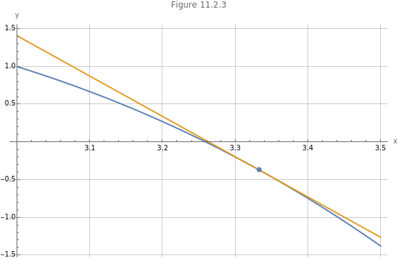
)In (7) we calculate the equation for the tangent line to at and graph the tangent line in Figure 10.2.3. The point of intersection of the tangent line with the axis is now even closer to the root of .
f
x
10
3
x
f
y
2
y
1
x
1
y
2
16
3
10
3
10
27
y
2
16
3
160
9
10
27
y
2
16
3
470
27
(
7
)ShowPlot-+2,-x+,x,3,,PlotLegends->"Expressions",PlotLabel->"Figure 10.2.3",AxesLabel->{"x","y"},GridLines->Automatic,ImageSize->Large,ListPlot,-
3
(x-2)
16
3
470
27
7
2
10
3
10
27
Out[]=
This is very close to the approximate root calculated below using the Solve function.
The function is a second-degree polynomial and we expect two roots. Figure 10.2.4 visualizes the two roots.
We can use our user-defined function to calculate a root.
To confirm our results, we use the Roots function.
Newton’s method can be used for functions that are not polynomials.
In this problem we cannot use the Roots function as it only take polynomials as parameter.
10.3 Optimization
10.3 Optimization
We create a user-defined function v below to represent the volume of the cylinder.
10.4 Optimization using numerical methods
10.4 Optimization using numerical methods
It is important to note that the minimum that we calculate with gradient descent might only be a local minimum and not a global minimum.
In the case of finding a maximum, we use the iterative process in (13).
In the code cell below we create a user-defined function gradientDescentSingle to perform the iterative process of gradient descent. The parameters are the function, the unknown variable, the learning rate, and the maximum number of iterations.
10.5 Numerical differentiation
10.5 Numerical differentiation
10.5.1 Definition of the derivate of a single variable function
10.5.1 Definition of the derivate of a single variable function
Not all derivatives of single variable functions can be solved analytically. Instead, we use the definition of the derivative to calculate a numerical approximation.
10.5.2 Numerical differentiation
10.5.2 Numerical differentiation
The values that we calculated for the derivative are indeed on the curve of the derivative itself.
Figure 10.5.2.8 visualizes the function and its derivative using the definition shown in the first line of (17).
Figure 10.5.2.9 shows the solution.