9 | THE BEHAVIOUR OF FUNCTIONS
9 | THE BEHAVIOUR OF FUNCTIONS
This chapter of Single Variable Calculus by Dr JH Klopper is licensed under an Attribution-NonCommercial-NoDerivatives 4.0 International Licence available at http://creativecommons.org/licenses/by-nc-nd/4.0/?ref=chooser-v1 .
9.1 Introduction
9.1 Introduction
In this chapter we investigate the very important topic of the behaviour of functions. In health data science we are often tasked with solving problems where the changes and properties of the curve of a function on an interval are extremely important to understand.
Figure 9.1.1 show the number of cases of a disease in a College dormitory on the time interval from day to day .
10
20
Plot[+10,{t,10,20},PlotRange->{{10,20},{0,100}},PlotLabel->"Figure 9.1.",AxesLabel->{"time","cases"},GridLines->Automatic,ImageSize->Large]
2
(t-12)
Out[]=

There is clearly a day-to-day change in the number of cases. It also seems as if the cases decrease in number from day to day , but then it increases again. These properties of the curve of the function in Figure 9.1.1 are the subject of exploration in this chapter.
10
12
9.2 Extrema
9.2 Extrema
While many single variable functions are defined over the whole set of real numbers, we are often interested in the behaviour of the function on an interval, which may only be a part of the domain of the function.
The interval is typically denoted by the letter and may be closed, indicated by the notation ], where , , and both and are included in the interval. The open interval does not include the values or , but all values between these boundary values.
I
[a,b
a,b∈
a<b
a
b
(a,b)
a
b
There are also semi-open or semi-closed intervals. The interval is left-closed and right open, with included in the interval but no , and the interval is left-closed and right-open, where is not included in the interval but is.
[a,b)
a
b
(a,b]
a
b
In the case of the curve of a single variable function , we plot the curve on a Cartesian plane, with on the horizontal axis and on the vertical axis. If the function is continuous everywhere on the interval then there is some value where is the maximum value on the horizontal axis (or it may the minimum value).
yf(x)
x
y
I[a,b]
a≤c≤b
f(c)
Definition 9.2.1 An extremum of a function which is continuous on some interval is a maximum or minimum value that the function reaches on an interval .
f(x)
I
I
We differentiate between a global and a local extrema.
Definition 9.2.2 A global extremum of a function which is continuous on some interval is the overall maximum or minimum on the interval, whereas a local extremum is the maximum or minimum on an interval contained within .
f(x)
I
J
I
Consider the function on the interval , shown in Figure 9.2.1.
y-+5
2
x
-,
1
2
1
2
ShowPlot-+5,x,-,,PlotRange->-,,{4.5,5.1},PlotLabel->"Figure 9.2.1",AxesLabel->{"x","y"},GridLines->Automatic,ImageSize->Large,GraphicsBlue,PointSize[0.02],Point,,Point-,
2
x
1
2
1
2
3
4
3
4
1
2
19
4
1
2
19
4
Out[]=
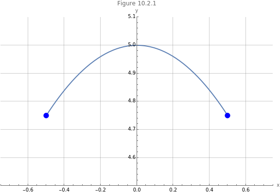
On this interval the function has a global minimum of at both and and a global maximum of .
19
4
x-
1
2
x
1
2
5
Now consider the same function on the open interval , shown in Figure 9.2.2.
-,
1
2
1
2
ShowListPlot-,,,,PlotMarkers"OpenMarkers",PlotRange->-,,{4.5,5.1},PlotLabel->"Figure 9.2.2",AxesLabel->{"x","y"},GridLines->Automatic,ImageSize->Large,Plot-+5,x,-,
1
2
19
4
1
2
19
4
3
4
3
4
2
x
1
2.02
1
2.02
Out[]=
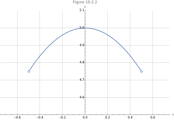
This function has a global maximum, but no global minima. The minima are reached for the limits as and , but these values of are not in the interval .
x-
1
2
x
1
2
x
I
Figure 9.2.3 shows the piecewise defined function in () on the open interval .
-,
1
2
1
2
f(x)=
|
(
1
)ShowListPlot-,,,,{0,5},PlotMarkers"OpenMarkers",PlotRange->-,,{4.5,5.1},PlotLabel->"Figure 9.2.2",AxesLabel->{"x","y"},GridLines->Automatic,ImageSize->Large,ListPlot0,,Plot-+5,x,-,-0.01,Plot-+5,x,0.01,
1
2
19
4
1
2
19
4
3
4
3
4
49
10
2
x
1
2.02
2
x
1
2.02
Out[]=

This function has no global extrema. The left- and right-hand limits as is , but the value of the function at is , which is smaller than .
x0
5
x=0
49
10
5
These definitions bring us to the following theorem.
Theorem 9.2.1 The extreme value theorem states that a function that is continuous on a closed interval has a maximum and a minimum on that interval.
f(x)
I
Next in our exploration is the concept of a critical point.
We use the D function to confirm the result.
Figure 9.2.4 visualizes the problem.
Before we graph the function, we follow the steps to calculate the extrema. We create a user-defined function f to solve the problem.
We calculate the values of the function at the boundaries of the interval.
Figure 9.2.5 visualizes our results.
9.3 Mean value theorem of differentiation
9.3 Mean value theorem of differentiation
We also note a tangent line which has the same slope as the secant line.
This property of a point with a tangent line with the same slope as the secant line is the mean value theorem of differentiation.
To do the calculation in (12) we create a user-defined function f.
We start with the secant line in ().
9.4 Increasing and decreasing functions
9.4 Increasing and decreasing functions
We use the mean value theorem Theorem 9.3.1 to write a theorem on the direction of a function in three parts.
We can use the sign of the slope on either side of a critical point to indicate if a point is a minimum or a maximum.
Problem 9.4.2 Find the critical values for the function in (16) and determine if the values are minima or maxima using the first-derivative test.
Using the second derivate, we have theorem for concavity.
We can use the inflection point in a theorem.
Figure 9.4.4 shows the inflection point. It is clear that the graph is concave down to the left of the infection point and concave up to the right of the inflection point.
From concavity follows the next theorem.
This is the second-derivative test.
From their model is seem that the number of cases decreases over time and then starts to increase again. It also seems that the rate of decrease increases until a certain point in time, before slowing down until the rate of decrease stops.
Determine the minimum number of cases in the given time interval and the time at which it occurs. Also determine the time when the rate of decrease is at its maximum.
We have to confirm that this is a minimum. It may be easy to see from Figure 9.4.4, but we should still confirm the result. This is down by looking the the sign of the second derivative at this time point.
We confirm this visually in Figure 9.4.5, where we plot the first derivative.