8 | IMPLICIT DIFFERENTIATION AND THE DERIVATIVES OF INVERSE FUNCTIONS
8 | IMPLICIT DIFFERENTIATION AND THE DERIVATIVES OF INVERSE FUNCTIONS
This chapter of Single Variable Calculus by Dr JH Klopper is licensed under an Attribution-NonCommercial-NoDerivatives 4.0 International Licence available at http://creativecommons.org/licenses/by-nc-nd/4.0/?ref=chooser-v1 .
8.1 Introduction
8.1 Introduction
All the functions and that we have encountered so far in this textbook have been explicit function, where we can write as a function of and then use formal techniques to solve the derivative symbolically.
y
x
Not all function can be written in explicit form. In this chapter we explore function that cannot be written in explicit form and develop a technique for solving for the first derivative of these functions.
The technique is fairly simple, but requires practice to master.
In the second part of the chapter we explore how to take the derivative of inverse functions, including the derivative of inverse trigonometric functions.
8.2 Implicit differentiation
8.2 Implicit differentiation
For some single variable functions we cannot explicitly write . Such function are implicit functions.
yf(x)
Definition 8.2.1 An implicit function of the independent variable is a function that does not explicitly express the dependent variable as a function .
x
y
f(x)
We might still be required to calculate the rate of change of with respect to .
y
x
Consider the function in (1) for which we would like to calculate (x).
′
y
y
e
(
1
)We cannot write as a function of . Instead we have to develop a method of implicit differentiation. Before we do so, we can use the properties of exponents and the natural logarithm, shown in (). We also have that , which we first encountered in chapter 5.
y
x
ln(e)=1
ln()=aln(b)
a
b
(
2
)The problem is rewritten in (), where we can write and a function of /
y
x
y
e
y
e
1
x
(
3
)We confirm this result using the . We also use the (x). We also use indexing notation as the result is a list of lists. The TraditionalForm function returns a result using mathematical typesetting.
D
function to calculate the derivative with respect to x
Solve
function to solve teh resultant derivative for ′
y
In[]:=
TraditionalForm[Solve[D[==x,x],y'[x]][[1,1]]]
y[x]
Out[]//TraditionalForm=
′
y
-y(x)
Note that the Wolfram Language as a function of . The result is which from the original implicit function is equal to as in our solution.
y
x
-y
e
1
x
We were fortunate that we could use the properties of the exponent and the logarithm to write as a function of , which is an explicit form.
y
x
The same problem, in implicit form, can also be solved using implicit differentiation. This technique consider as a function of and the derivative of any term that contains is managed by the chain rule. The technique is shown in () for x where we take the first derivative with respect to on both sides and use Leibniz notation initially.
y
x
y
y
e
x
d
dx
y
e
d
dx
y
e
dy
dx
dy
dx
1
y
e
1
x
(
4
)In the second step of (4), we treat as a variable and the first derivative of with respect to is . Because we are using the chain rule, we have to differentiate with respect to as well.
y
y
e
y
y
e
y
x
Problem 8.2.1 Calculate the first derivative of with respect to of the equation in ().
y
x
2
x
2
y
(
5
)This equation for a circle with radius can be rewritten in explicit form, shown in ().
2
2
y
2
x
4-
2
x
(
6
)The derivative with respect to of this explicit function can be calculated individually for the positive and negative square roots, using the chain rule, shown in (). We only consider . If we included the negative square root we no longer have a function as we break to horizontal rule test.
x
+
4-
2
x
y=y'=(-2x)y'=-y'=-
4-
y=2
x
1
2
(4-)
2
x
1
2
-
1
2
(4-)
2
x
x
4-
2
x
x
y
(
7
)The solution is shown in () using implicit differentiation.
2x+2y=02y=-2xy=-x=-
dy
dx
dy
dx
dy
dx
dy
dx
x
y
(
8
)The code below confirms the result.
In[]:=
TraditionalForm[Solve[D[+==4,x],y'[x]][[1,1]]]
2
x
2
y[x]
Out[]//TraditionalForm=
′
y
x
y(x)
Figure 8.2.1 shows the semicircle .
y+
4-
2
x
Plot
4-
,{x,-2,2},PlotLabel->"8.2.1",AxesLabel->{"x","y"},GridLines->Automatic,ImageSize->Large,AspectRatio->Automatic2
x
Out[]=

At the point we have that . The slope at the point ) is given by the solution and is shown in ().
x=1
y=
3
(1,
3
m=f'(x)===
-x
y
-1
3
-
3
3
(
9
)Using the equation for the point-slope form of an equation, we calculate an equation for a line through the given point and with the given slope, shown in ().
y-=m(x-)y=(x-1)+
y
1
x
1
-
3
3
3
(
10
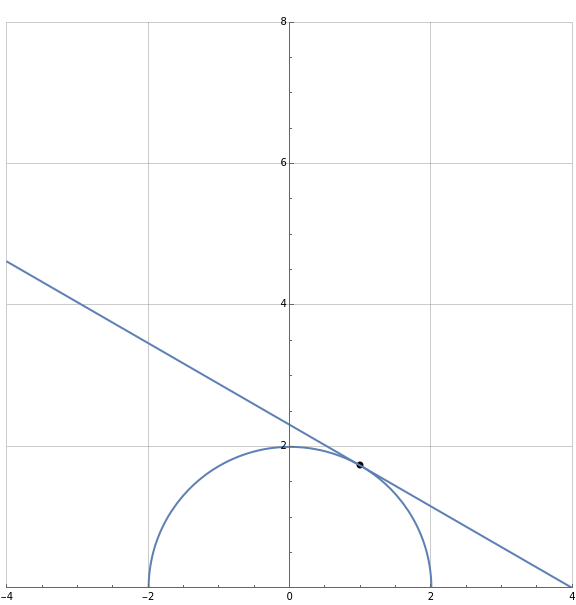
)Figure 8.2.2 show the graph of the function, then given point and the tangent line to the curve at the point.
ShowPlot(x-1)+
4-
,{x,-2,2},PlotRange->{{-4,4},{4,4}},PlotLabel->"Figure 8.2.2",AspectRatio->Automatic,GridLines->Automatic,ImageSize->Large,Graphics[PointSize[Large],Point[1,2
x
3
]],Plot-
3
3
3
,{x,-4,4}Out[]=
Implicit differentiation is best mastered by completing example problems.
The solution is shown in (12).
The code below confirms the result.
In some problems we have to use the product rule and the chain rule.
The code below confirms the result.
We use product and chain rules in (16).
The code below confirms the result.
The solution follows in (18).
The code below confirms the result.
We van take the natural logarithm on both sides to solve the problem, shown in (18).
The code below confirms the result.
We confirm the result using the D function.
To complete the following problem we remember the properties of logarithms shown in (23), together with the property in (2).
While the function in the next problem is in explicit form, we can now solve it using implicit differentiation.
Instead of using the product, quotient, and the chain rules, we will use implicit differentiation
We take the natural logarithm of both sides in (25). The function is then in implicit form and we use implicit differentiation after using the properties of logarithms.
The code below confirms the result, where the Wolfram Language has expanded the product of terms.
We can also solve functions with trigonometric functions that are defined implicitly.
We have to make use of the product and chain rules to use implicit differentiation in the problem. The result follows in (27).
The code below confirms the result, where the Wolfram Language has expanded the product of terms.
The solution follows in (29).
The code below confirms the result, where the Wolfram Language has expanded the product of terms.
The solution follows in (31).
The code below confirms the result, where the Wolfram Language has expanded the product of terms.
8.3 Derivatives of inverse functions
8.3 Derivatives of inverse functions
A function that is one-to-one passes the horizontal line test. The horizontal line test states that the curve of a function does not intersect any horizontal line more than once on a specified interval.
To confirm that the function are indeed inverse of each other, we verify that (33) holds, as shown in (35).
The D function is used to confirm our result. We use the ArcSin function as first parameter.
Similar arguments can be used for other trigonometric functions. We use the Wolfram Language to show the first derivatives of the inverse of the cosine and the inverse of the tangent functions.