7 | SERIES EXPANSION AND APPROXIMATIONS
7 | SERIES EXPANSION AND APPROXIMATIONS
This chapter of Single Variable Calculus by Dr JH Klopper is licensed under an Attribution-NonCommercial-NoDerivatives 4.0 International Licence available at http://creativecommons.org/licenses/by-nc-nd/4.0/?ref=chooser-v1 .
7.1 Introduction
7.1 Introduction
In this chapter we explore the series expansion of functions. The Maclaurin series is a special case of Taylor expansions. Such expansions allow us to recreate functions within an interval. This helps us understand the approximation of functions.
7.2 Higher-order derivatives
7.2 Higher-order derivatives
7.3 Maclaurin series
7.3 Maclaurin series
7.4 Taylor series
7.4 Taylor series
The Taylor series expansion of a function is the generalization of the Maclaurin series at .
f(x)
x
x
0
Definition 7.4.1 The Taylor series is an infinite expansion of a function at , given in ().
f(x)
x
x
0
f(x)=+++()+…f(x)=()
f()
x
0
0
(x-)
x
0
0!
f'()
x
0
1
(x-)
x
0
1!
f''()
x
0
2
(x-)
x
0
2!
(3)
f
x
0
3
(x-)
x
0
3!
lim
n->∞
n
∑
i=0
(i)
f
x
0
i
(x-)
x
0
i!
(
17
)We can once again truncate the expansion to the -order derivative, shown in ().
th
n
f(x)‶+++()+…+()+O
f()
x
0
0
(x-)
x
0
0!
f'()
x
0
1
(x-)
x
0
1!
f''()
x
0
2
(x-)
x
0
2!
(3)
f
x
0
3
(x-)
x
0
3!
(n)
f
x
0
n
(x-)
x
0
n!
n+1
(x-)
x
0
(
18
)
Problem 7.4.1 Calculate the Taylor series expansion of the function at to the fifth order derivative.
f(x)
x
e
x4
In () we calculate , and the derivatives with respect to at .
f(4)
x
x4
f(x)=andf(4)=f'(x)=andf'(4)=⋮(x)=and=
x
e
4
e
x
e
4
e
(5)
f
x
e
(5)
f
4
e
(
19
)In () we use the calculation above and the definition of the Taylor series to calculate the solution.
f(x)≈++++++Of(x)≈1+(x-4)+++++O
4
e
0
(x-4)
0!
4
e
1
(x-4)
1!
4
e
2
(x-4)
2!
4
e
3
(x-4)
3!
4
e
4
(x-4)
4!
4
e
5
(x-4)
5!
6
(x-4)
4
e
2
(x-4)
2
3
(x-4)
6
4
(x-4)
24
5
(x-4)
120
6
(x-4)
(
20
)The code below confirms the result. Note that the Wolfram Language result does not extract as a common factor.
4
e
In[]:=
Series[,{x,4,5}]
x
Out[]=
4
4
1
2
4
2
(x-4)
1
6
4
3
(x-4)
1
24
4
4
(x-4)
1
120
4
5
(x-4)
6
O[x-4]
7.5 Linear approximation
7.5 Linear approximation
In () we consider the point-slope form of a line in the Cartesian plane tangent to a curve at =a, where with and , the function of the tangent line.
f(x)
x
1
m=f'(a)
(,)=(a,f(a))
x
1
y
1
y=L(x)
y-=m(x-)y=m(x-)+L(x)=(x-a)f'(a)+f(a)
y
1
x
1
x
1
y
1
(
21
)In () we consider the function at =1, where =f(1)==1 with and .
f(x)=
2
x
x
1
y
1
2
1
f'(x)=2x
f'(1)=2
L(x)=(x-1)(2)+1L(x)=2x-2+1L(x)=2x-1
(
22
)This is the function for the tangent line at .
L(x)
(,)(1,1)
x
1
y
1
Figure 7.5.1 visualizes the curve and the tangent line at .
f(x)
2
x
L(x)
(,)(1,1)
x
1
y
1
ShowPlot{,2x-1},x,,,PlotLegends->{"curve of the function","linear approximation"},PlotLabel->"Figure 7.5.1",AxesLabel->{"x","y"},GridLines->Automatic,ImageSize->Large,Graphics[{PointSize[Large],Point[{1,1}]}]
2
x
6
10
3
2
Out[]=
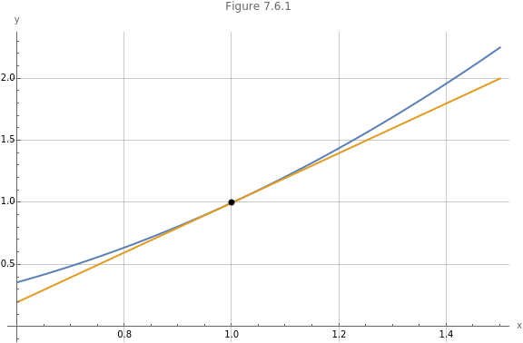
The tangent line approximates the curve at and is called a linear approximation.
x=1
Definition 7.5.1 The linear approximation of a function at is the function of the tangent line at , shown in ().
f(x)
xa
L(x)≈f(x)
xa
L(x)=(x-a)f'(a)+f(a)
(
23
)We can calculate the interval on which the difference between the function and its linear approximation less than (or equal to) a given value. In the code cell below, we create the user-defined functions f and tangent to hold the original function in the example above and its linear approximation at .
x=1
In[]:=
f[x_]:=tangent[x_]:=2x-1
2
x
The code considers where the difference between the function and its linear approximation is less than a tenth. We use the RealAbs function since the difference is a distance and should not be sign dependent. The TraditionalForm function prints the results in mathematical format.
In[]:=
TraditionalFormRealAbs[f[x]-tangent[x]]<
1
10
Out[]//TraditionalForm=
-2x+1<
2
x
1
10
The Reduce function calculates the interval.
In[]:=
TraditionalFormReduceRealAbs[f[x]-tangent[x]]<,x
1
10
Out[]//TraditionalForm=
1
10
10
)<x<1
10
10
)Using the N function, we can calculate a linear approximation to the domain.
In[]:=
NTraditionalFormReduceRealAbs[f[x]-tangent[x]]<,x
1
10
Out[]//TraditionalForm=
0.683772<x<1.31623
The inequality of fairly simple to solve by hand. First, we factor the expression -2x+1 which is the difference between the function and its linear approximation in().
2
x
2
x
2
(x-1)
(
24
)The factorization is confirmed using code.
In[]:=
Factor[-2x+1]
2
x
Out[]=
2
(-1+x)
We solve the inequality for in ().
x
<<x-1<-<x-1<+1<x<+1-+1<x<+1-+<x<+(10-(
2
(x-1)
1
10
2
(x-1)
1
10
1
10
1
10
1
10
(expansionoftheinequality)
-1
10
1
10
1
10
1
10
10
10
10
10
10
10
10
10
1
10
10
)<x<1
10
10
+10)(
25
)
Problem 7.5.1 Calculate a linear approximation of the function near .
L(x)
f(x)+
x
x=4
The result is shown in ().
We use the same code as in the explanation of linear approximations above to solve the problem.
We use the definition of the linear approximation in ().
We plot the solution in Figure 7.5.3.
7.6 Approximation using series expansion
7.6 Approximation using series expansion
By using the Maclaurin series expansion, and more generally the Taylor series expansion, we can calculate approximations that are closer to the original function on a larger domain.
Below we calculate terms up to the eight derivative.