We expand in (1-r) for IR boundary behaviour (both variables and their derivatives) for the NDSolve (this isn’t strictly necessary but gives us polynomial rather than logarithmically defined BC’s).
which satisfy the UV behaviour which is V=Log[r] and W=Log[r]. These will be used to fix the boundary conditions in the numerical equation solver. They are also used to calculate the temperature.
In[]:=
u
1
[B_]:=
u
1
[B]=Module[{},u1v/.FindRoot[{vsol[
r
UV
,B,u1v,w0v]-Log[
r
UV
]0,wsol[
r
UV
,B,u1v,w0v]-Log[
r
UV
]0},{{u1v,0.1},{w0v,0.1}}]]//Quiet
w
0
[B_]:=
w
0
[B]=Module[{},w0v/.FindRoot[{vsol[
r
UV
,B,u1v,w0v]-Log[
r
UV
]0,wsol[
r
UV
,B,u1v,w0v]-Log[
r
UV
]0},{{u1v,0.1},{w0v,0.1}}]]//Quiettemp[B_]:=
u
1
[B]
4π
Define the renormalised action from which the limit of the cutoff is taken to
r
UV
to give us the final action which will be used below to calculate the Gibbs Free energy.
Here we include the data from the last calculation (gibbsdatalistplot) so that you don’t have to run it. This is the plot of
G/
4
T
versus
B/
2
T
that we will use for the rest of the calculations.
In[]:=
gibbsdatalist=Cases
,Point[__],Infinity[[1,1]];
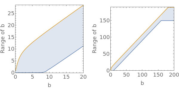
We are going to fit to the data in gibbsdatalist using a polynomial, but the data range that we use for the fitting will depend on the value of b. We will be taking data from between lower[b] and upper[b]. These functions are not particularly carefully chosen, but just found to have a reasonable shape.
This function takes the data from gibbsdatalist in the region dictated by lower and upper above
Define the renormalised gibbs density given by subtracting the quadratic piece.
This function fits the data to a sixth order polynomial in the range around the value of b
Here we define the magnetisation, entropy, susceptibility and pressures along with their renormalised counterparts
Define the region that we want to do most of the plots in
First the magnetisation minus the magnetisation at T=114 MeV
The subtracted susceptibility at a range of magnetic field values as a function of T.
The specific heat as a function of T.
The speeds of sound as a function of T for different values of the magnetic field.
The subtracted speeds of sound at T=150 and 300 MeV as a function of B
Comparison to lattice data
Here we take data from author = {Bali, G. S. and Bruckmann, F. and Endrodi, G. and Katz, S. D. and Schafer, A.}, title = “{The QCD equation of state in background magnetic fields}”, eprint = “1406.0269”, archivePrefix = “arXiv”, primaryClass = “hep-lat”, doi = “10.1007/JHEP08(2014)177”, journal = “JHEP”, volume = “08”, pages = “177”, year = “2014” where we have plotted various physical quantities and compare our results with these lattice results.