MAM2046W - Second year nonlinear dynamics
MAM2046W - Second year nonlinear dynamics
Section 3.5: Coupled oscillators and quasiperiodicity
Section 3.5: Coupled oscillators and quasiperiodicity
When we discussed the phase space of the pendulum in first year, we said that we were free to choose and (0), which is indeed true, but we ended up plotting trajectories in phase space like:
θ(0)
θ
In[]:=
xsol[t_,xv_]:=Module[{},sol=NDSolve[{x''[t]+Sin[x[t]]0,x[0]0,x'[0]xv},x,{t,0,100}][[1]];{x[t],x'[t]}/.sol];ParametricPlot[Evaluate[xsol[t,#]&/@Range[0,2.5,0.25]],{t,0,100},PlotRange->{{-3,10},{-3,3}},AspectRatio->1/2,AxesLabel->{Style["(t)",18],Style["(t)",18]},ImageSize->600]
x
1
x
2
Out[]=
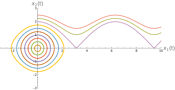
(where here isθ and is ). We never took into account the fact that θ is periodic (though is of course not) - ie . The way we should do this is to acknowledge that the phase plane shouldn’t be but it should be × - ie a cylinder.
x
1
x
2
θ
θ
θ+2πisidentifiedwithθ
2
1
1
S
In[]:=
xsol[t_,xv_]:=Module[{},sol=NDSolve[{x''[t]+Sin[x[t]]0,x[0]0,x'[0]xv},x,{t,0,100}][[1]];{x[t],x'[t]}/.sol];Evaluate[xsol[t,#]&/@Range[0,2.5,0.25]];TableParametricPlot3D[Evaluate[{Cos[#[[1]]],Sin[#[[1]]],#[[2]]}&/@%],{t,0,100},ViewPointRotationTransform[θ,{0,0,1}][{3,0,1}]],θ,0,2π,;ListAnimate[%,SaveDefinitions->True,AnimationRunTime->10]
2π
20
Out[]=

Imagine taking the first plot and pasting it around a cylinder of circumference 2π.
OK, so here we have an example when a phase plane is most naturally described as a phase cylinder. Are there other systems for which we might have a different description?
We know that in a one dimensional system we can’t have any oscillations in terms of a back and forth motion, but of course we can have a flow on the line, where there is an identification on the line meaning that it’s really on a circle. Such a flow would be given by:
θ
where the ∼ symbol means “is identified with”. This is really a flow on a circle.
We can do the same thing in two dimensions, and think about having two coupled oscillators (flows on a circle), given by, for instance
θ
1
ω
1
K
1
θ
2
θ
1
θ
2
ω
2
K
2
θ
1
θ
2
Where andarethe natural frequencies of the motion (ie. without the terms we would just have going around a circle at frequency ), and are coupling constants. We see then that when and are very close to each other, or differ by π, the couplings are small, and when they differ by or the couplings are large. This system wants to keep the closetoeach other, or exactly out of phase. Both the live on a circle. We can plot them on the same circle and see their trajectory. For instance if we start with =1, =5 and both =1we get:
ω
1
ω
2
K
i
θ
i
ω
i
K
i
θ
1
θ
2
π
2
3π
2
θ
i
θ
i
ω
1
ω
2
K
i
In[]:=
{θ1[t],θ2[t]}/.NDSolve[{θ1'[t]==1+Sin[θ2[t]-θ1[t]],θ2'[t]==5+Sin[θ1[t]-θ2[t]],θ1[0]==0,θ2[0]==0.5},{θ1,θ2},{t,0,20}][[1]];Table[Show[ListPlot[Evaluate[Evaluate[{{Sin[%[[#]]],Cos[%[[#]]]}}]],PlotRange->{{-2,2},{-2,2}},PlotStyle->{{Red,PointSize[0.02]},{Blue,PointSize[0.02]}}[[#]]]&/@{1,2},Graphics[Circle[{0,0},1]],ImageSize->500,AspectRatio->1],{t,0,3,0.1}];ListAnimate[%,SaveDefinitions->True]
Out[]=
Is there a simpler way that we could illustrate this? We normally like to think about the state of a system as a single point in phase space. The problem with the above is that we have a single state as being given by two points on the circle. The issue is that we have a two dimensional phase space and we are trying to represent it on a one dimensional space. So what we really need is a space with two compact directions. Such a space is the torus. In the above, we have a state given by two points The torus is a surface which is parameterised by So for two points on the circle corresponds to a single point on the surface of the torus.
((t),(t)).
θ
1
θ
2
((t),(t)).
θ
1
θ
2
The torus is actually given by the product space ×, which is like having two independent circles. One way to see this is to take a piece of paper and first identify the left and right opposite sides. You’ve now got one circular direction. Now do the same thing with the top and bottom (actually, this will be hard with paper as it’s not stretchable) and you have two circular directions.
1
S
1
S
Taking the above system of two positions on the circle converting them to one position on the torus, we get the following trajectory:
(,)and
θ
1
θ
2
In[]:=
{θ1[t],θ2[t]}/.NDSolve[{θ1'[t]==1+Sin[θ2[t]-θ1[t]],θ2'[t]==5+Sin[θ1[t]-θ2[t]],θ1[0]==0,θ2[0]==0.5},{θ1,θ2},{t,0,20}][[1]];Table[Show[ParametricPlot3D[{Cos[t](2+Cos[u]),Sin[t](2+Cos[u]),Sin[u]},{t,0,2Pi},{u,0,2Pi},PlotStyle->Opacity[0.5],PlotRange->All,Mesh->False],ListPointPlot3D[{{Cos[%[[2]]](2+Cos[%[[1]]]),Sin[%[[2]]](2+Cos[%[[1]]]),Sin[%[[1]]]}}/.t->t1,PlotStyle->Blue],ParametricPlot3D[{Cos[%[[2]]](2+Cos[%[[1]]]),Sin[%[[2]]](2+Cos[%[[1]]]),Sin[%[[1]]]}/.t->t2,{t2,0,t1},PlotStyle->Red]],{t1,0.1,10,1}];ListAnimate[%,SaveDefinitions->True]
Out[]=

This particular case is an example of a general form of a vector field which lives on a torus. That of
Going back to the coupled oscillator, there are a couple of interesting limits we can look in.
The first is to ask what happens if the system is not coupled at all. Well, then we get two particles moving around the circle at their own rate, say 1:
Clearly if they are both moving at the same rate, then not only is each particle's trajectory periodic with period 2π, but in fact after 2π, the whole system is back to where it started. How about where we have
well, here, although the first has period π and the second has period 2π, it takes 2π for the whole system to get back to where it started, although the first oscillator has been around twice by this point. What about if we had
Plotting this on the torus we see:
The path that the trajectory makes on the torus is the so-called trefoil knot, which, if we turn the trajectory into a tube to make it easier to visualise, looks like:
In fact we can make a more general statement. If we have two frequencies
Somehow we have a system where the natural frequency is given by the difference between the original frequencies, and the new “coupling” is additive in the old couplings.
What do we do when we are looking at dynamical systems? We ask about the fixed points! The fixed points are clearly given by
Well, this only has solutions when
In fact there will be exactly two fixed points for
and only one when
Which looks very much look a saddlenode bifurcation...I rephrase...it is a saddlenode bifurcation.
Thankfully both give the same frequency of
we have the following trajectories
If we have
then there is no fixed point, and no phase locking. You can see here that the lines keep crossing each other.
The boundary between the phase locked dynamics and the non phased locked dynamics is a saddlenode bifurcation of cycles.