Exercises 3.4.c
Exercises 3.4.c
For:=x-rx(1-x)
x
i) Sketch the different vector field types that appear when you vary .
r
We can actually get some intuition here before drawing any graphs. To find the fixed points, just solve
x-rx(1-x)=0
for which gives:
x
x=0andx=
r-1
r
So before we even plot a phase portrait we can get the bifurcation diagram. We need to be able to figure out along the fixed point lines what is going to be stable and what unstable. Let’s look at the fixed point first and do a linear stability analysis. Close to is approximated by:
x=0
x=0,theequation
x
(as the is approximated by just 1 close to We know that this has solutions:
1-x
x=0).
x=
x
0
(1-r)t
e
and therefore if this is an unstable solution if then it’s stable.
(1-r)>0⟹r<1
r>1
For completeness, let’s expand the equation also about the other fixed point: Let
x=.
r-1
r
x=+η:
r-1
r
η
r-1
r
r-1
r
r-1
r
which, after some algebra actually gives the much simpler looking:
η
2
η
which, for small η gives
η
and we have exactly the opposite situation than we had for the first fixed point. ie. and is unstable. Let’s plot these two solutions
r<1isstable
r>1
In[]:=
ShowPlot0,,{r,-2,1},PlotStyle->{{Blue,Dashed},Blue},Plot0,,{r,1,2},PlotStyle->{Blue,{Blue,Dashed}},PlotRange->{All,{-3,5}},PlotRange->{All,{-3,5}},AspectRatio->1,AxesLabelEvaluate[Style[#,18]&/@{"r","x"}]
r-1
r
r-1
r
Out[]=

OK, so we should also be drawing the phase portrait for this. We can do this the old fashioned way by just plotting the graph of the differential equation for different values of r:
Which, while there’s a fixed point which is doing some funky things around , just has a single bifurcation at .
r=0
r=1
In[]:=
ga[pos_]:=Graphics[{Thick,Arrowheads[0.05],Arrow[pos]}]pl1=GraphicsGridPartitionShowPlot[x-#x(1-x),{x,-4,4},PlotRange->{{-4,4},{-2,2}},AxesLabelEvaluate[Style[#,14]&/@{"x",""}],AspectRatio->1,PlotLabel->Style["r = "<>ToString[#],14],PlotStyle->Blue],If#<0,Showga[{{0,0},{-2,0}}],ga{0,0},,0,ga{4,0},,0,Graphics[Circle[{0,0},0.1]],GraphicsDisk,0,0.1,If#==0,Show[ga[{{0,0},{-2,0}}],ga[{{0,0},{2,0}}],Graphics[Circle[{0,0},0.1]]],If#<1,Showga{-2,0},,0,ga{0,0},,0,ga,0,{2,0},Graphics[Circle[{0,0},0.1]],GraphicsDisk,0,0.1,If#==1,Show[ga[{{-2,0},{0,0}}],ga[{{0,0},{2,0}}]],Showga[{{-2,0},{0,0}}],ga,0,{0,0},ga,0,{2,0},Graphics[Disk[{0,0},0.1]],GraphicsCircle,0,0.1&/@Range[-1,4,0.5],3,ImageSize->800
x
#-1
#
#-1
#
#-1
#
#-1
#
#-1
#
#-1
#
#-1
#
#-1
#
#-1
#
#-1
#
Out[]=
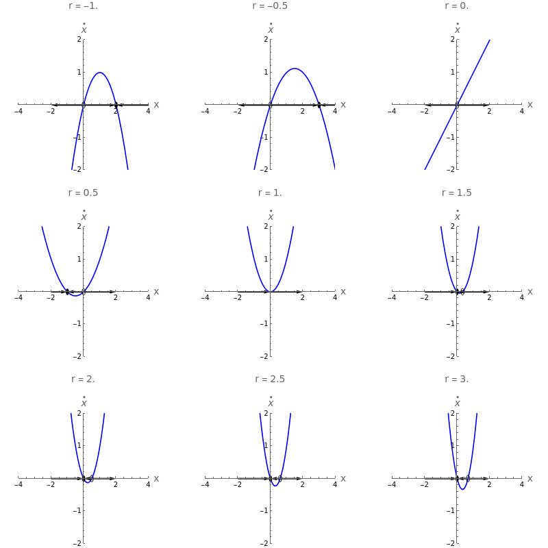
Which ties in with our bifurcation plot. Now we just need to make sure that we can convert it into the Normal Form for a transcritical bifurcation. The equation is:
x
Expanding in
xthisisjust:
x
2
x
Dividing through by -r gives:
-=x-
1
r
x
(r-1)
r
2
x
Now let
R=⟹r=
r-1
r
1
1-R
which gives us
(R-1)=Rx-
x
2
x
Now the left hand side is really
(R-1)
dx
dt
and so defining this gives us finally:
T=t⟶(R-1)=(R-1)=
1
(R-1)
dx
dt
dx
dT
dT
dt
(R-1)
(R-1)
dx
dT
Which is the normal form of a transcritical bifurcation.