Section 3.3: Transcritical Bifurcations
Section 3.3: Transcritical Bifurcations
Transcritical Bifurcations
That's a bit of a mouthful, but we'll see that this isn't any more complicated than previous examples. One example where this occurs is in population dynamics.
Imagine that you have a species in some environment. Clearly there will always be a fixed point at zero population, whatever the dynamics of the system. However, whether or not this is a stable or unstable fixed point can vary. Sometimes if you have a very small population it will die out, and in other situations, if you have a very small population it can grow exponentially. Remember we spoke about the logistic equation for population growth which is:
P
P
M
We're going to look at a slightly simpler equation which is:
x
2
x
(Notice that this is equivalent to the logistic equation with and )
k=M=r
x=P
Actually, we should pause for a moment and discuss the examples we’ve been looking at. These “prototypical examples”, like “=rx- ”, and “ =+r ” are called normal forms. You can think of them as the most basic example that exhibits a particular type of bifurcation. Actually there is a lot more to them than that, but that’s the best way to think of them for now. You will see in the exercises for part 3 why they are important.
x
2
x
x
2
x
So, where are the fixed points of this system? The normal form in this case is “ =rx- ”, which can also be written as =x(r- ), so clearly is always going to be a fixed point. But there will be another at . Let’s plot the situations with separately.
x
2
x
x
x
x=0
x=r
r<0,r=0,r>0
In[]:=
ploptions={AxesLabel{Style["x",14],Style["",14]},AxesOrigin{0,0},PlotRange{-1.5,1},AspectRatio0.5};pla=Show[Plot[-x-,{x,-2,2},Evaluate[ploptions]],Graphics[Arrow[#]]&/@{{{-1.2,0},{-1.75,0}},{{-0.8,0},{-0.25,0}},{{0.8,0},{0.25,0}}},Graphics[Circle[{-1,0},0.1]],Graphics[Disk[{0,0},0.1]],PlotLabelStyle["r<0",14]];plb=ShowPlot[-,{x,-2,2},Evaluate[ploptions]],Graphics[Arrow[#]]&/@{{{-0.5,0},{-1.5,0}},{{1.5,0},{0.5,0}}},Graphics[Circle[{0,0},0.1]],GraphicsDisk{0,0},0.1,,,AxesOrigin{0,0},PlotLabelStyle["r=0",14];plc=Show[Plot[x-,{x,-2,2},Evaluate[ploptions]],Graphics[Arrow[#]]&/@{{{-0.25,0},{-0.8,0}},{{0.25,0},{0.8,0}},{{1.8,0},{1.25,0}}},Graphics[Circle[{0,0},0.1]],Graphics[Disk[{1,0},0.1]],PlotLabelStyle["r>0",14]];GraphicsGrid[{{pla,plb,plc}},ImageSize1000,Spacings-100]
x
2
x
2
x
3π
2
5π
2
2
x
Out[]=
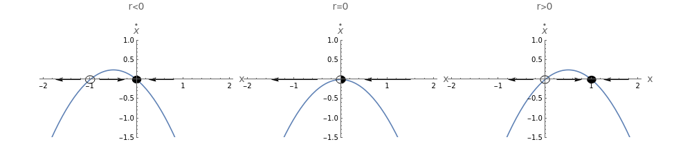
We see that as we increase the value of the fixed point at moves from being stable, to half-stable to unstable. and the other fixed point goes from being unstable, to merging into the central fixed point, to being stable. We can plot these fixed points on the following bifurcation diagram. Dashed lines again correspond to unstable fixed points, and solid lines are stable fixed points.
r
x=0
In[]:=
Show[Plot[{r,0},{r,0,1},PlotStyle{{Thickness0.01,Black},{Thickness0.01,Black,Dashing0.05}},PlotRange{{-1,1},{-1,1}},AxesLabel(Style[#,20]&/@{"r","x"}),AspectRatio1],Plot[{0,r},{r,-1,0},PlotStyle{{Thickness0.01,Black},{Thickness0.01,Black,Dashing0.05}},PlotRange{{-1,1},{-1,1}},AxesLabel(Style[#,20]&/@{"r","x"}),AspectRatio1]]
Out[]=
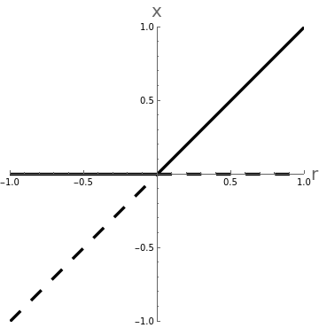
The sweeping fixed point swings from one direction, coalesces with the other, and they exchange stability's. Where the dashed lines are again unstable fixed points and the solid lines are stable. You can see, as you increase the fixed point at zero going from stable to unstable. As the stable and unstable fixed points come together we get a semi-stable fixed point.
r
Of course, in the example of a population, you can never have a negative population, so the unstable fixed point at negative (or ) would never show up physically, but a stable fixed point at zero can shift to an unstable fixed point at zero and a stable fixed point if the carrying capacity changes sign.
x
P
Note that it’s not always the case that this change happens at . It can happen at any point.
x=0
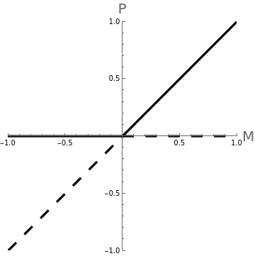
Going back to the example of population dynamics, the carrying capacity can be thought of as the parameter which varies. If you have a positive carrying capacity, then is an unstable fixed point, but if it’s negative it becomes a stable fixed point.
P=0
In this case, if you naively plotted the bifurcation diagram it would look like:
In[]:=
Show[Plot[{r,0},{r,0,1},PlotStyle{{Thickness0.01,Black},{Thickness0.01,Black,Dashing0.05}},PlotRange{{-1,1},{-1,1}},AxesLabel(Style[#,20]&/@{"M","P"}),AspectRatio1],Plot[{0,r},{r,-1,0},PlotStyle{{Thickness0.01,Black},{Thickness0.01,Black,Dashing0.05}},PlotRange{{-1,1},{-1,1}},AxesLabel(Style[#,20]&/@{"P","M"}),AspectRatio1]]
Out[]=
but clearly a negative population doesn’t make any sense, so the physically interesting part of this diagram looks like:
In[]:=
ShowPlot{r,0},{r,0,1},PlotStyle{{Thickness0.01,Black},{Thickness0.01,Black,Dashing0.05}},PlotRange{{-1,1},{-0.1,1}},AxesLabel(Style[#,20]&/@{"M","P"}),AspectRatio,Plot[0,{r,-1,0},PlotStyle{Thickness0.01,Black},PlotRange{{-1,1},{-0.1,1}},AxesLabel(Style[#,20]&/@{"P","M"}),AspectRatio1]
1
2
Out[]=
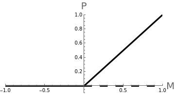
This tells us that a population would die out when if it is governed by the logistic equation.
M<0
Let’s look at another example of a system which includes a transcritical bifurcation:
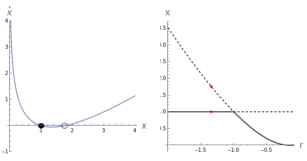
x
It’s clear here that , is always a fixed point of the system, but for there is also another fixed point. Let’s look at this system as we change . In the following picture, you see that as changes, for the phase portrait on the left and the bifurcation diagram on the right.
x=1
r<0
r
r
In[]:=
sol[r_]:=x/.NSolve[rLog[x]+x-10,x]//Quietpl1=Show[Plot[sol[r][[1]],{r,-2,-0.1},PlotStyle{Black}],Plot[sol[r][[2]],{r,-2,-0.1},PlotStyle{Black,Dashed}],PlotRangeAll];tab=Table[Labeled[GraphicsGrid[{{Show[Plot[rLog[x]+x-1,{x,0,4},PlotRange{-1,4},AxesLabel(Style[#,18]&/@{"x",""})],Graphics[Disk[{sol[r][[1]],0},0.1]],Graphics[Circle[{sol[r][[2]],0},0.1]],AspectRatio1],Show[pl1,ListPlot[{r,#}&/@sol[r],PlotStyle{Red,PointSize[0.02]}],AxesLabel(Style[#,18]&/@{"r","x"}),AspectRatio1]}}],"r = "<>ToString[r]],{r,-2,-0.1,0.11}];ListAnimate[tab,SaveDefinitionsTrue]
x
Out[]=
Our equation is:
And we are left with:
Important Note: Don’t let this example intimidate you! I know it looks complicated, and you might think it’s crazy how different it looks from start to finish, but really take time to step through it. Once you’ve do the exercise at the end, check it with the lecturer and see where you can improve. This kind of manipulation becomes incredibly important as you move forward and acing it now will set you on the right path!
This is the important point about a normal form. ALL saddle node bifurcations, close to the point where the bifurcation happens can be turned into the form:
by a change of variables, and ALL transcritical bifurcations can be put into the form:
by an appropriate change of variables.
Give it a go yourself. Draw the bifurcation diagram for the equation:
and put this equation into normal form via a change of variables.