Hyperdimensional Computing and the Dollar of Mexico

Hyperdimensional computing (HDC) is an emerging paradigm in artificial intelligence that leverages the power of high-dimensional vectors, called hypervectors, to encode and manipulate data. Unlike conventional computing approaches that rely on precise numerical calculations, HDC employs distributed and approximate representations, making it highly fault-tolerant.

In this notebook we will use bipolar and binary hypervectors—large vectors composed of either bipolar elements (+1s and -1s) or binary elements (0s and 1s) . Their high dimensionality (e.g., 10,000 bits) allows for efficient representation of complex patterns while ensuring robustness to noise and errors.

We will illustrate how HDC can encode and manipulate complex relationships using the classic example introduced by Pentti Kanerva in the paper: What We Mean When We Say "What's the Dollar of Mexico?": Prototypes and Mapping in Concept Space.

Bipolar Hypervectors

{-1,1}

are mathematically convenient for vector arithmetic. They allow efficient dot product computations and can be easily adapted to standard linear algebra operations implementations.

A bipolar hypervector would be like :

In[]:=

RandomChoice[{-1,1},10000]//Short(*notedimension=10,000*)

Out[]//Short=

{1,-1,1,1,1,1,1,1,1,1,1,-1,9977,-1,1,1,1,-1,-1,1,1,1,1,-1}

An interesting and useful property of hyperspace is that randomly created vectors are more likely perpendicular to each other (almost).

For bipolar vectors, a common metric for the similarity between two hypervectors is their normalized scalar product. This is also called cosine similarity:

In[]:=

similarity[vs1_,vs2_]:=N[Normalize[vs1].Normalize[vs2]]

With this measure of similarity, we can verify that randomly created hypervectors are almost orthogonal (≈0) to each other :

In[]:=

{vs1,vs2}=RandomChoice[{-1,1},{2,10000}];

In[]:=

similarity[vs1,vs2]

Out[]=

0.0048

To illustrate this further we compare the distribution of similarities between random vectors in 10 dimension on one hand, and in between hypervectors on the other hand :

In[]:=

v=RandomChoice[{-1,1},10];

In[]:=

PairedHistogram[Table[similarity[v,RandomChoice[{-1,1},10]],{1000}],Table[similarity[vs1,RandomChoice[{-1,1},10000]],{1000}]]

Out[]=

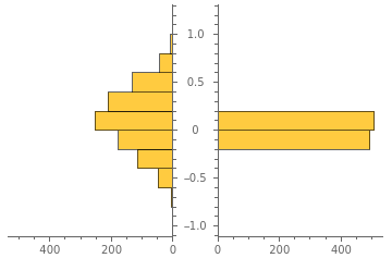
Notice that most HDVs are approximately orthogonal to one another.

This property is due to the high dimensionality of the space and not to the nature of the vector as we will verify later with binary vectors.

Next we introduce two key operations in HDC, Bundling and Binding. They represent the addition and multiplication of this vector algebra. A third operation, Permutation – a shifting or scrambling operation that introduces order sensitivity into the representations, will not be treated here.

Bundling with addition

Bundling or aggregation, also called superposition, combines two o more HDVs in a new HDV that is similar to all of its constituents. A majority-rule operation that combines multiple vectors into a single representation, akin to a form of associative memory. For bipolar vectors this is typically achieved through element-wise addition, elementwise normalized to [-1,1].

If you add an even number of bipolar vectors, some components will end up 0. We’ll replace that 0 with 1 or -1 randomly. This will add a little bit of unintentional but also unimportant background noise :

In[]:=

bundle[hdv__]:=Clip[Plus[hdv]]/.x_/;x==0:>RandomChoice[{-1,1}]

Let’s bundle three hypervectors:

In[]:=

{hpv1,hpv2,hpv3}=RandomChoice[{-1,1},{3,10000}];

In[]:=

vsum=bundle[hpv1+hpv2+hpv3];

and compare the similarities

In[]:=

similarity[vsum,#]&/@{hpv1,hpv2,hpv3}//N

Out[]=

{0.5028,0.5038,0.4966}

As shown above, the result of bundling is a vector that is equally similar ( ≈ 0.5 ) to each of its constituents.

Binding with multiplication

Binding is a fundamental operation in HDC that combines two hypervectors to create a new hypervector that is dissimilar to both input vectors. This operation is commonly used to “associate” information, for instance, to assign values to variables.

For bipolar hypervectors, binding is typically implemented as element-wise multiplication. We can verify that the resulting vector is dissimilar to both input vectors :

In[]:=

similarity[vs1*vs2,#]&/@{vs1,vs2}//N

Out[]=

{-0.0076,-0.002}

Binding is commutative and distributive over the bundling operation. This is easy to see because binding and bundling are just bitwise multiplication and addition. But binding also preserves similarity relationships between vectors. For a quick check we start with two similar vectors :

In[]:=

similarity[vsum,vs1]

Out[]=

0.0078

Create a new random hypervector to bind to each of these vectors and check similarity :

In[]:=

vs3=RandomChoice[{-1,1},10000];

In[]:=

similarity[vs3*vsum,vs3*vs1]

Out[]=

0.0078

Similarity is indeed preserved.

Also bipolar vectors are their own multiplicative inverse:

In[]:=

vs1*vs1*vs2==vs1*vs2*vs1==vs2

Out[]=

True

What is the ‘Dollar of Mexico’?

And here it is! This is the main example in this notebook, taken from Pentti Kanerva's paper which it is refered for an explanation.

We start generating random hypervectors to represent each entity that we’ll use: • Countries: USA, MEX (USA and Mexico) • Capitals: WDC, MXC (Washington DC, Mexico City) • Monies: DOL, PES (Dollar, Peso) • Roles: NAM, CAP, MON (Name, Capital, Money)

In[]:=

{NAM,CAP,MON,USA,MEX,WDC,MXC,DOL,PES}=RandomChoice[{-1,1},{9,10000}];

We then create composite representations for each country:

In[]:=

USTATES=bundle[NAM*USA+CAP*WDC+MON*DOL];

In[]:=

MEXICO=bundle[NAM*MEX+CAP*MXC+MON*PES];

And bind this together to make a new vector that represents our database :

In[]:=

F=USTATES*MEXICO;

To answer “What is the Dollar of Mexico?”, we perform:

In[]:=

query=DOL*F;

The resulting hypervector will be most similar to the query effectively answering the question :

In[]:=

similarity[query,#]&/@{NAM,CAP,MON,USA,MEX,WDC,MXC,DOL,PES}

Out[]=

{-0.0062,0.0106,0.001,0.01,-0.001,-0.005,-0.0116,-0.0018,0.2328}

The last entry in the list above has the highest similarity and correspond to the hypervector PES.

But now that we know what we’re doing, we can do much better. We can use a build-in vector database for this example:

In[]:=

database=CreateVectorDatabase[{NAM->"Name",CAP->"Capital",MON->"Money",USA->"USA",MEX->"Mexico",WDC->"Whashington DC",MXC->"Mexico City",DOL->"The Dollar",PES->"El Peso"},DistanceFunction->CosineDistance];

Notice the option DistanceFunction -> CosineDistance is appropriate.

Then we can query the database for “The Dollar of Mexico”.

In[]:=

VectorDatabaseSearch[database,query]

Out[]=

{El Peso}

Binary Hypervectors

Binary Hypervectors {0,1} are often manipulated using bitwise operations, making them highly hardware-efficient and well-suited for digital implementations. Operations like XOR (exclusive OR) and majority-rule addition enable powerful algebraic transformations for encoding and reasoning.

A binary hypervector would be like :

In[]:=

v=RandomInteger[1,10000];v//Short

Out[]//Short=

{0,0,1,0,1,1,0,0,0,1,0,0,1,9974,1,1,1,0,1,1,0,1,1,0,1,0,0}

A similarity measure commonly used for binary dense vectors is the complementary Hamming distance. Hamming distance, named after Richard Hamming, is a measure of the difference between two strings of equal length. It counts the number of positions at which the corresponding symbols differ, essentially quantifying the minimum number of substitutions required to change one string into another.

In[]:=

hammingSimilarity[hdv1_,hdv2_]:=1-2HammingDistance[hdv1,hdv2]/Length[hdv1]

And then we can illustrate the histogram of the similarities:

In[]:=

Histogram[Table[hammingSimilarity[v,RandomInteger[1,10000]],{1000}]]

Out[]=

The histogram shows that most binary hypervectors are very dissimilar/perpendicular (similarity≈0) to each other. It was the same with bipolar vectors before.

Bundling binaries

Bundling for binary hypervectors is again addition and normalization to [0, 1] bitwise. Also there is an adjustment to make when a component has the same value as the threshold used to determined when to set a component to 1 or 0. We set those randomly.

We can verify the similarity of a bundled vector with its constituents :

We see that the bundled vector is about equally similar to all its constituents.

Binding binaries

For binary hypervectors {1,0} the binding of two hypervectors is performed through a bitwise Xor operation :

We can verify that the binding of two hypervectors is indeed dissimilar to its constituents :

The Dollar of Mexico again

We start creating our binary hypervectors and build our dataset:

And to perform the query :

In the list above, one pick the vector of most similarity, the vector PES as before.

We conclude using the built-in vector database for binary hypervectors this time using the option DistanceFunction -> HammingDistance :