2020 Solution 06
2020 Solution 06
Total jitter (Tj) is calculated by the following formula.
Tj = Dj + QBER Rj
Where,
Tj is the total jitter
Dj is the deterministic jitter component
Rj is the random jitter component
QBER is a multiplier.
Tj = Dj + QBER Rj
Where,
Tj is the total jitter
Dj is the deterministic jitter component
Rj is the random jitter component
QBER is a multiplier.
Choose the best response to the following statement.
"Peak to peak random jitter will vary with the number of samples."
"Peak to peak random jitter will vary with the number of samples."
(a) True. Random jitter is "unbounded", with tails in the distribution. Therefore measured pk-to-pk values will change with the number of samples.
(b) False
(c) Indeterminate
(d) Unlikely
(e) Likely
(f) .......
(b) False
(c) Indeterminate
(d) Unlikely
(e) Likely
(f) .......
Verify
Verify
The following is a trivial verification. First generate a list of random numbers.
In[]:=
myRandomNumbers=RandomVariate[NormalDistribution[0,0.3],10^3];
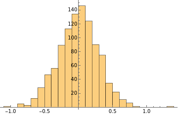
It is essential to to verify that the dataset meets the expectations about boundedness. Plot the dataset to see if it looks like a Gaussian distribution with tails.
In[]:=
Histogram[myRandomNumbers,AxesOrigin{0,0},PlotRangeAll]
Out[]=
Pick up random samples of varying lengths from the list of random numbers. You will see three sublists with 20, 50 and 80 elements.
In[]:=
randomSamples=RandomSample[myRandomNumbers,#]&/@{20,50,80}
Out[]=
{{0.143469,0.33215,-0.0933257,-0.00717707,-0.44774,0.477221,0.141959,-0.120462,0.0682826,0.1866,0.394421,-0.0262532,0.14604,-0.140918,0.646917,0.0272508,0.674578,-0.468153,0.165312,-0.118361},{0.611546,-0.127389,-0.167028,-0.0819431,-0.113884,0.141233,-0.358543,0.3892,0.374876,0.205589,-0.547886,0.296499,0.159787,-0.116407,0.0471571,0.232443,-0.298479,-0.142546,-0.0392723,0.232682,-0.0273524,0.00667336,0.137234,-0.238624,-0.325941,0.111439,-0.586394,0.362974,-0.29943,0.101678,0.411517,0.18324,-0.032499,-0.521616,-0.307438,-0.0100416,-0.0467681,0.180776,-0.26121,0.146324,0.173702,0.100197,-0.157089,0.506017,-0.245983,0.0484572,-0.426327,-0.00965429,0.159299,0.0375794},{0.0490753,-0.157289,0.139494,0.319027,-0.215311,-0.0569092,-0.0529944,0.395318,-0.063641,-0.440002,-0.384882,0.0385878,-0.130095,0.437084,0.0933442,0.236701,0.0756806,-0.538021,-0.307438,0.118944,0.21126,0.326494,0.153812,0.0883184,-0.418382,-0.150329,0.571329,0.0371754,-0.0167733,-0.553166,-0.342943,-0.377584,-0.0341578,0.296499,0.0652008,0.353415,0.313709,-0.133556,0.50361,0.341605,0.306505,0.44596,0.0913112,-0.20209,-0.013103,-0.127389,0.248897,0.119589,-0.327647,0.217366,-0.134043,-0.0103086,0.027102,-0.348384,-0.315566,0.37618,-0.216593,-0.608052,-0.251285,0.13965,0.0375794,-0.0433797,-0.310569,0.18324,-0.670764,-0.554966,-0.0707858,-0.345559,0.18966,-0.294505,0.031725,-0.132071,0.13022,0.224113,-0.237211,-0.242634,0.6817,0.224452,0.255429,0.257515}}
Test each sublist to find the peak-to-peak value within that sublist. Does it vary with the number of elements sampled? The result is of the form {no.of samples, pk-pk}.
In[]:=
samplesPkpk={Length@#,Max[#]-Min[#]}&/@randomSamples
Out[]=
{{20,1.14273},{50,1.19794},{80,1.35246}}
Its always a good idea to plot.
In[]:=
ListPlot[samplesPkpk,FrameTrue,FrameStyle16,FrameLabel{"Samples, n","pk-pk, Unitless"},GridLinesAutomatic]
Out[]=
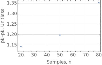
The peak-to-peak value varies with the number of samples.